10. Predictive models: prep, train, test, and evaluate • Text as Data Resources

Overview

In this Recipe we will build a predictive model that will work as a spam filter. The data we will work with are SMS (Short Message Service) text messages from the SMS Spam Collection (Almeida and G’omez Hildago 2011). The process steps will include preparing the dataset, splitting it into training and testing sets, building a training model, testing the model, and evaluating the results. We will use the Quanteda package (Benoit et al. 2022) as it is a package that facilitates preparing, modeling, and exploring text models.

Let’s load the packages we will use in this Recipe.

library(tidyverse)           # data manipulation
library(quanteda)            # tokenization and document-frequency matrices
library(quanteda.textstats)  # descriptive text statistics
library(quanteda.textmodels) # naive bayes classifier

Coding strategies

Orientation

Let’s first read in a become familiar with the SMS dataset. We can access this dataset through the tadr package.

sms_df <- tadr::sms  # load dataset from tadr package
glimpse(sms_df)  # preview dataset structure

## Rows: 5,574
## Columns: 2
## $ sms_type <chr> "ham", "ham", "spam", "ham", "ham", "spam", "ham", "ham", "sp…
## $ message  <chr> "Go until jurong point, crazy.. Available only in bugis n gre…

The sms_df object is a data frame with 5,574 observations and two columns. The observations correspond to individual text messages. sms_type reflects the type of SMS message; either legitimate (‘ham’) or spam and the message contains the message text.

In this recipe I will be suffixing the object names to reflect the object type. We will work with our dataset in four main formats: data frame (_df), corpus _corpus, tokens _tokens, and document-frequency matrix (_dfm).

Let’s see the proportion of spam to ham messages in our dataset. I will use the tabyl() function from the janitor package to get the counts and proportions.

sms_df %>%
    janitor::tabyl(sms_type)

sms_type	n	percent
ham	4827	0.866
spam	747	0.134

So now we know a majority of the messages are ‘ham’, around 87% to be exact.

Preparation

We will now create a Quanteda corpus object our of our sms_df data frame. A corpus object is a complex R object which will allow us to manipulate the data and maintain metadata in an accessible format. To create a corpus object all we need to do is call the corpus() function and set the text_field argument to identify the column where the text is.

sms_corpus <- # quanteda corpus object
  corpus(sms_df, # data frame
         text_field = "message") # text field

sms_corpus %>% 
  summary(n = 5) # preview corpus object

Text	Types	Tokens	Sentences	sms_type
text1	22	29	3	ham
text2	7	12	2	ham
text3	33	37	2	spam
text4	10	17	2	ham
text5	13	14	1	ham

The summary() function provides an overview of the dataset including some calculated text statistics (‘Types’, ‘Tokens’, and ‘Sentences’) as well as metadata. In corpus objects the metadata is known as document variables, or ‘docvars’. We can access the document variables directly with the docvars() function.

sms_corpus %>% # corpus object
  docvars() %>%  # get corpus metadata attributes
  slice_head(n = 5) # first observations

sms_type
ham
ham
spam
ham
ham

We can add metadata to our corpus object by simply making reference to a new column and assigning values to it. In our data we are going to want to have a unique document id for each of our 5,574 text messages. We want to create a vector of numbers 1 to 5,574. One way to do this is by using the 1:5574 syntax with the number hardcoded in. Another more flexible way to create the document id vector that is exactly fit to the number of observations is by using the ndoc() function on the corpus object itself. ndoc() will return the number of documents in the corpus object. For corpus objects observations are known as documents and for us a document is a text message.

sms_corpus$doc_id <- # create a new column `doc_id`
  1:ndoc(sms_corpus) # add numeric id to each text message

We can now look at the document variables again and we will see that the doc_id column now appears.

sms_corpus %>% # corpus object
  docvars() %>%  # get corpus metadata attributes
  slice_head(n = 5) # first observations

sms_type	doc_id
ham	1
ham	2
spam	3
ham	4
ham	5

Of note, if at any time we would like to convert our corpus object back into a data frame we can use the tidy() function from the tidytext package.

sms_corpus %>% # corpus object
  tidytext::tidy() %>% # convert back to a data frame
  slice_head(n = 5) # first observations

text	sms_type	doc_id
Go until jurong point, crazy.. Available only in bugis n great world la e buffet… Cine there got amore wat…	ham	1
Ok lar… Joking wif u oni…	ham	2
Free entry in 2 a wkly comp to win FA Cup final tkts 21st May 2005. Text FA to 87121 to receive entry question(std txt rate)T&C’s apply 08452810075over18’s	spam	3
U dun say so early hor… U c already then say…	ham	4
Nah I don’t think he goes to usf, he lives around here though	ham	5

Feature engineering

The next step towards preparing our dataset for use in the predictive model is to decide what the features are that will be used to help the predictive model learn how to distinguish between spam and ham text messages. To create language features we will tokenize the text into smaller linguistic units. We can choose from characters, words, or sentences, or ngram sequences of either characters or words. For many predictive models, the default feature to select as a starting point will be words. However, if there is reason to believe that some other linguistic unit(s) would make more practical sense there is nothing limiting you from selecting another unit. If we later see that the model does not perform well we can always come back and tweak the tokenization process and try other linguistic units.

Let’s move forward by tokenizing the messages into words. We will also remove punctuation and numbers and lowercase all the messages. The tokens() function allows us to do all but lowercasing.

sms_tokens <- 
  tokens(x = sms_corpus, # corpus object
         what = "word", # tokenize by words
         remove_punct = TRUE, # remove punctuation
         remove_numbers = FALSE) # remove numbers

The result assigned to sms_tokens is a ‘tokens’ object. Looking a the first few messages we can see that they have been tokenized into words.

sms_tokens %>%
    head(n = 5)  # preview first 5 tokenized messages

## Tokens consisting of 5 documents and 2 docvars.
## text1 :
##  [1] "Go"        "until"     "jurong"    "point"     "crazy"     "Available"
##  [7] "only"      "in"        "bugis"     "n"         "great"     "world"    
## [ ... and 8 more ]
## 
## text2 :
## [1] "Ok"     "lar"    "Joking" "wif"    "u"      "oni"   
## 
## text3 :
##  [1] "Free"  "entry" "in"    "2"     "a"     "wkly"  "comp"  "to"    "win"  
## [10] "FA"    "Cup"   "final"
## [ ... and 20 more ]
## 
## text4 :
##  [1] "U"       "dun"     "say"     "so"      "early"   "hor"     "U"      
##  [8] "c"       "already" "then"    "say"    
## 
## text5 :
##  [1] "Nah"    "I"      "don't"  "think"  "he"     "goes"   "to"     "usf"   
##  [9] "he"     "lives"  "around" "here"  
## [ ... and 1 more ]

The head() function has been used here instead of the slice_head() function we have typically used. It is of note that head() works much like slice_head() with the main distinction that slice_head() only works on data frame objects where head() will work on any type of R object. In this case sms_tokens is a ‘tokens’ object which is a more complex type of list object.

What is nice about a tokens object is that the metadata from the corpus object sms_corpus is retained. We can preview the metadata again with docvars().

sms_tokens %>% 
  docvars() %>%  # get corpus metadata attributes
  slice_head(n = 5) # first observations

sms_type	doc_id
ham	1
ham	2
spam	3
ham	4
ham	5

It is good to know that these document variables can be used to group (tokens_group()), subset (tokens_subset()), and sample (tokens_sample()) the sms_tokens object much like functions from the tidyverse package when working with data frames.

There are a number of other functions which can be used to manipulate the tokens themselves inside the tokens object (tokens_ngrams(), tokens_toupper(), etc.). For our purposes we will use one of these functions named tokens_tolower() which will lowercase all the tokens.

sms_tokens <- 
  sms_tokens %>% # 
  tokens_tolower() # lowercase all characters

sms_tokens %>% 
  head(n = 5) # preview first 5 tokenized messages

## Tokens consisting of 5 documents and 2 docvars.
## text1 :
##  [1] "go"        "until"     "jurong"    "point"     "crazy"     "available"
##  [7] "only"      "in"        "bugis"     "n"         "great"     "world"    
## [ ... and 8 more ]
## 
## text2 :
## [1] "ok"     "lar"    "joking" "wif"    "u"      "oni"   
## 
## text3 :
##  [1] "free"  "entry" "in"    "2"     "a"     "wkly"  "comp"  "to"    "win"  
## [10] "fa"    "cup"   "final"
## [ ... and 20 more ]
## 
## text4 :
##  [1] "u"       "dun"     "say"     "so"      "early"   "hor"     "u"      
##  [8] "c"       "already" "then"    "say"    
## 
## text5 :
##  [1] "nah"    "i"      "don't"  "think"  "he"     "goes"   "to"     "usf"   
##  [9] "he"     "lives"  "around" "here"  
## [ ... and 1 more ]

Now we have our tokens ready that we will use as features in our prediction model.

The next step is to create a Document-Frequency Matrix (DFM). In this structure each unique token has a column and each unique document a row. The values are the (raw) counts of each of the tokens for each of the documents. To create a DFM we use the dfm() function.

sms_dfm <- dfm(sms_tokens)  # create a document-frequency matrix

sms_dfm %>%
    head(n = 5)  # preview first 5 documents in the dfm

## Document-feature matrix of: 5 documents, 9,313 features (99.84% sparse) and 2 docvars.
##        features
## docs    go until jurong point crazy available only in bugis n
##   text1  1     1      1     1     1         1    1  1     1 1
##   text2  0     0      0     0     0         0    0  0     0 0
##   text3  0     0      0     0     0         0    0  1     0 0
##   text4  0     0      0     0     0         0    0  0     0 0
##   text5  0     0      0     0     0         0    0  0     0 0
## [ reached max_nfeat ... 9,303 more features ]

The preview shows some key information about our sms_dfm object. Our preview only contains 5 documents, but 9,313 features. The features are the number of unique tokens in the matrix. Each document will have the number of times each unique token appeared in a message as a value. Since only a subset of the 9,313 possible feature tokens will appear in any given message this means that may values will be 0. The relative amount of zeros to non-zeros is called sparsity. In the preview we also see that our matrix is 99.84% sparse. This is not uncommon but in cases where there the features number in the 10s of thousands (also not uncommon) the matrix will become quite large and incur processing and memory costs that may need to be taken into account.

Our matrix is not unwieldly at it’s current size so we won’t ‘trim’ it, but it is good to know that quanteda provides a dfm_trim() function that can be used to trim features that either do not have a certain frequency count threshold (usually minimum frequency min_termfreq =) or are sparse (column-wise) to a certain percentage (sparsity =).

Let’s explore the features in our DFM. We can use the topfeatures() function to retrieve the most frequent features in the sms_dfm object.

sms_dfm %>%
    topfeatures(n = 10)

##    i   to  you    a  the    u  and   is   in   me 
## 2298 2252 2145 1446 1335 1168  979  895  891  800

We can also use the textstat_frequency() function from the quanteda.textstats package to get frequency measures as well as group these statistics by a document variable. In this case let’s look at the frequency statistics for both spam and ham SMS types.

sms_dfm %>% 
  textstat_frequency(n = 5, # get top 5 features
                     groups = sms_type) # group by sms_type

feature	frequency	rank	docfreq	group
i	2252	1	1609	ham
you	1855	2	1295	ham
to	1562	3	1219	ham
the	1131	4	867	ham
a	1067	5	883	ham
to	690	1	467	spam
a	379	2	295	spam
call	346	3	319	spam
£	324	4	253	spam
you	290	5	238	spam

We can see that our grouped frequency statistics show similarities and differences. On the one hand we can see that the frequency counts and document frequency are much larger for ham. This makes sense since around 87% of the messages are ham in our dataset. On the other hand, if we look at particular features we see that ‘i’ is the most common feature for ham and ‘to’ for spam. There is some overlap as well ‘you’ and ‘a’ appear in both ham and spam. The more overlap we have between features the less distinctive our classes (ham and spam) will be which can make it more difficult for the prediction model to make accurate predictions.

For the moment we will continue to move forward and see how the model does despite these similarities, but it is important to know that we can apply some techniques to reduce similarity. One way is to return to our tokenization process and remove common words using a stopword list. This approach is common but relies on pre-defined lists of what is considered common. Another approach is to weigh the distribution of the given dataset such that the number of documents in which a feature appears in influences the feature value. This weighting is called the Term Frequency-Inverse Document Frequency (TF-IDF). We can use the dfm_tfidf() function to transform the sms_dfm matrix and view how this weighting effects our apparent overlap in top features for ham and spam.

sms_dfm %>% 
  dfm_tfidf() %>% # calculate term frequency-inverse document frequency weighted scores
  textstat_frequency(n = 5, # get top 5 features
                     groups = sms_type, # group by sms_type
                     force = TRUE) # force calculation despite weights

feature	frequency	rank	docfreq	group
i	1193	1	1609	ham
you	1040	2	1295	ham
u	834	3	702	ham
the	828	4	867	ham
to	811	5	1219	ham
£	432	1	253	spam
to	358	2	467	spam
call	351	3	319	spam
free	305	4	168	spam
your	258	5	227	spam

We can see now that the TF-IDF scores have reduced the apparent overlap. Let’s keep this in mind when we evaluate our model performance. For now we will continue with the raw counts as our value scores.

The last step we need to do to prepare our dataset for predictive modeling is to split the dataset into training and testing sets. The training set should contain around 75% of the dataset and the other 25% will be reserve for testing. Both datasets should have similar relative proportions of the classes we want to predict (i.e. ham and spam).

Let’s create a numeric vector which we will use to randomly sample 75% of the observations from our sms_dfm for use in training. First I will set a random number seed set.seed() to make this example reproducible. Next I will calculate the number of documents in the sms_dfm with the ndoc() function. then I will multiply this number by .75 to get the sample size we want. The we can use the sample() function to get the train_ids. Note we set replace = FALSE so no ids are repeated in the sample (all 75% will be unique).

set.seed(300) # make reproducible

num_docs <- 
  sms_dfm %>% # dfm object
  ndoc() # get number of documents

train_size <- 
  (num_docs * .75) %>% # get size of sample
  round() # round to nearest whole number

train_ids <- sample(x = 1:num_docs, # population
                   size = train_size, # size of sample
                   replace = FALSE) # without replacement

train_ids %>% head(n = 10)

##  [1] 2638  874 3650 3740  789  553 1705 4368 4557 2828

With our training ids train_ids we can now subset the sms_dfm into a training set and a test set.

sms_dfm_train <- 
  sms_dfm %>% # dfm object
  dfm_subset(doc_id %in% train_ids) # subset matching doc_id and train_ids

sms_dfm_test <- 
  sms_dfm %>% # dfm object
  dfm_subset(!doc_id %in% train_ids) # subset non-matching doc_id and train_ids

Let’s verify that the proportions of ham to spam are similar between the sms_dfm_train and sms_dfm_test sets. Again, I will use the tabyl() function.

sms_dfm %>% # dfm object
  docvars() %>% # pull the document variables
  janitor::tabyl(sms_type) # check ham/spam proportions

sms_type	n	percent
ham	4827	0.866
spam	747	0.134

sms_dfm_train %>% # dfm object
  docvars() %>% # pull the document variables
  janitor::tabyl(sms_type) # check ham/spam proportions

sms_type	n	percent
ham	3626	0.867
spam	554	0.133

sms_dfm_test %>% # dfm object
  docvars() %>% # pull the document variables
  janitor::tabyl(sms_type) # check ham/spam proportions

sms_type	n	percent
ham	1201	0.862
spam	193	0.138

The splits look comparable so we are good to proceed to training our prediction model.

Model training

We will be using a Naive Bayes Classifier algorithm implemented in the quanteda.textmodels package textmodel_nb(). Naive Bayes is a common starting algorithm for text classification. To train our model we need to pass the sms_dfm_train document-feature matrix which contains the values for each of our feature tokens to x and then the class labels (‘ham’ and ‘spam’) for each document using the document variables of the sms_dfm_train object. We will assign the model to nb1 and use summary() to see an overview of the training results.

nb1 <- 
  textmodel_nb(x = sms_dfm_train, # document-feature matrix
               y = sms_dfm_train$sms_type) # class labels

summary(nb1) # model summary

## 
## Call:
## textmodel_nb.dfm(x = sms_dfm_train, y = sms_dfm_train$sms_type)
## 
## Class Priors:
## (showing first 2 elements)
##  ham spam 
##  0.5  0.5 
## 
## Estimated Feature Scores:
##           go    until   jurong    point   crazy available    only     in
## ham  0.00323 0.000308 3.24e-05 1.62e-04 0.00013  0.000195 0.00159 0.0100
## spam 0.00104 0.000260 4.33e-05 4.33e-05 0.00026  0.000173 0.00303 0.0023
##         bugis       n    great    world       la        e   buffet     cine
## ham  1.14e-04 0.00180 0.001282 4.38e-04 9.73e-05 0.000973 3.24e-05 9.73e-05
## spam 4.33e-05 0.00039 0.000476 4.33e-05 4.33e-05 0.000217 4.33e-05 4.33e-05
##        there      got    amore      wat       ok      lar   joking      wif
## ham  0.00219 0.002920 3.24e-05 1.22e-03 0.003585 4.87e-04 6.49e-05 3.57e-04
## spam 0.00052 0.000217 4.33e-05 8.66e-05 0.000173 4.33e-05 4.33e-05 4.33e-05
##            u      oni     free    entry       2      a
## ham  0.01293 6.49e-05 0.000811 1.62e-05 0.00396 0.0133
## spam 0.00533 4.33e-05 0.007233 8.66e-04 0.00585 0.0118

In the nb1 model summary we see the ‘Call’, the ‘Class Priors’ and a preview of the ‘Estimated Feature Scores’. The class priors are set to 50/50 for ham and spam which means our model does not assume one class is more prevalent than the other. We will leave it this way as we don’t want to bias our model towards one class over the other –even though our input data is biased. The posterior probabilities for the features can be seen in the estimated feature scores. For a given word we can see how the model weighs individual features towards ham or spam. Our predictions will be based on the sum of these probabilities for the features of each text message in the testing dataset. We can see, for example, the probability of ‘u’ is higher for ham and ‘free’ leans towards ‘spam’. A feature like ‘a’, however, does not have much discriminatory power as it is split quite equally.

We can explore more of the feature probabilities using the coef() function on the nb1 model.

coef(nb1) %>% # get the feature coefficient scores
  head # preview the feature coefficient scores

##                ham     spam
## go        3.23e-03 1.04e-03
## until     3.08e-04 2.60e-04
## jurong    3.24e-05 4.33e-05
## point     1.62e-04 4.33e-05
## crazy     1.30e-04 2.60e-04
## available 1.95e-04 1.73e-04

We can also see the prediction scores for each document.

predict(nb1, type = "prob") %>% # get the predicted document scores
  head # preview predicted probability scores

##            ham     spam
## text1 1.00e+00 2.25e-08
## text2 1.00e+00 9.58e-05
## text3 3.31e-27 1.00e+00
## text4 1.00e+00 1.23e-08
## text5 1.00e+00 1.66e-11
## text6 5.94e-04 9.99e-01

With the prediction scores for each document, we can transform it so that we can subsequently join the actual class labels for the training dataset. There’s a lot going on in the code below, but the goal is to get model’s prediction for each document in the training dataset and include the model’s probability score.

nb1_predictions <- 
  predict(nb1, type = "prob") %>% # get the predicted document scores
  as.data.frame() %>% # convert to data frame
  mutate(document = rownames(.)) %>% # add the document names to the data frame
  as_tibble() %>% # convert to tibble
  pivot_longer(cols = c("ham", "spam"), # convert from wide to long format
               names_to = "prediction", # new column for ham/spam predictions
               values_to = "probability") %>% # probablity scores for each
  group_by(document) %>% # group parameter by document
  slice_max(probability, n = 1) %>% # keep the document row with highest probablity
  slice_head(n = 1) %>% # for predictions that were 50/50 
  ungroup() %>% # remove grouping parameter
  mutate(doc_id = str_remove(document, "text") %>% as.numeric) %>% # clean up document column so it matches doc_id in
  arrange(doc_id) # order by doc_id

nb1_predictions %>% 
  slice_head(n = 10) # preview

document	prediction	probability	doc_id
text1	ham	1.000	1
text2	ham	1.000	2
text3	spam	1.000	3
text4	ham	1.000	4
text5	ham	1.000	5
text6	spam	0.999	6
text7	ham	1.000	7
text8	ham	1.000	8
text9	spam	1.000	9
text10	spam	1.000	10

Now with nb1_predictions we can bind the column nb1$y from the model which contains all of the actual (original) class labels with the predictions.

nb1_predictions_actual <- 
  cbind(actual = nb1$y, nb1_predictions) %>% # column-bind actual classes
  select(doc_id, document, actual, prediction, probability) # organize variables

nb1_predictions_actual %>% 
  slice_head(n = 5) # preview

doc_id	document	actual	prediction	probability
1	text1	ham	ham	1
2	text2	ham	ham	1
3	text3	spam	spam	1
4	text4	ham	ham	1
5	text5	ham	ham	1

Now we can cross-tabulate actual and prediction with table() and send the results to the confusionMatrix() function from the caret package to provide a summary of the model’s performance on the training dataset.

tab_class <- 
  table(nb1_predictions_actual$actual, # actual class labels
        nb1_predictions_actual$prediction) # predicted class labels

caret::confusionMatrix(tab_class, mode = "prec_recall") # model performance statistics

## Confusion Matrix and Statistics
## 
##       
##         ham spam
##   ham  3582   44
##   spam   18  536
##                                         
##                Accuracy : 0.985         
##                  95% CI : (0.981, 0.989)
##     No Information Rate : 0.861         
##     P-Value [Acc > NIR] : <2e-16        
##                                         
##                   Kappa : 0.937         
##                                         
##  Mcnemar's Test P-Value : 0.0015        
##                                         
##               Precision : 0.988         
##                  Recall : 0.995         
##                      F1 : 0.991         
##              Prevalence : 0.861         
##          Detection Rate : 0.857         
##    Detection Prevalence : 0.867         
##       Balanced Accuracy : 0.960         
##                                         
##        'Positive' Class : ham           
##

So our trained model has a very high accuracy score on the data it was trained on. It’s not perfect, but in practice no algorithm will be. The question now how well this trained model will perform on the new dataset (sms_dfm_test). Let’s now move to test and then evaluate our model’s perform on the sms_dfm_train dataset.

Model testing

To test the model we first ensure that the features from the training and test datasets are matched with dfm_matched(). The we use the function predict() to use the nb1 model to predict the classes for the sms_dfm_train dataset without the class labels.

dfm_matched <- 
  dfm_match(sms_dfm_test, # test dfm
            features = featnames(nb1$x)) # (left) join with trained model features

predicted_class <- 
  predict(nb1, # trained model
          newdata = dfm_matched) # classify test dataset

Evaluation

Let’s now evaluate how well our model performs on the testing dataset.

actual_class <- dfm_matched$sms_type  # get actual class labels

tab_class <- table(actual_class, predicted_class)  # cross-tabulate actual and predicted class labels

caret::confusionMatrix(tab_class, mode = "prec_recall")  # model performance statistics

## Confusion Matrix and Statistics
## 
##             predicted_class
## actual_class  ham spam
##         ham  1161   40
##         spam    6  187
##                                         
##                Accuracy : 0.967         
##                  95% CI : (0.956, 0.976)
##     No Information Rate : 0.837         
##     P-Value [Acc > NIR] : < 2e-16       
##                                         
##                   Kappa : 0.871         
##                                         
##  Mcnemar's Test P-Value : 1.14e-06      
##                                         
##               Precision : 0.967         
##                  Recall : 0.995         
##                      F1 : 0.981         
##              Prevalence : 0.837         
##          Detection Rate : 0.833         
##    Detection Prevalence : 0.862         
##       Balanced Accuracy : 0.909         
##                                         
##        'Positive' Class : ham           
##

So we see that the trained nb1 model does quite well at 96.7% accuracy. If we dig into the cross-tabulation we see that the errors tend to be more for cases when the model predicts that messages are spam when they are in fact ham.

Let’s describe in more detail where the key statistics come from and how they are calculated. Below we have a summary of the meanings of the statistics:

Accuracy: measure of overall correct predictions
Precision: measure of the quality of the predictions
- Percentage of predicted ‘ham’ messages that were correct
Recall: measure of the quantity of the predictions
- Percentage of actual ‘ham’ messages that were correct
F1-score: summarizes the balance between precision and recall

To calculate these statistic by hand it is helpful to be able to read a confusion matrix as seen in Figure 1.

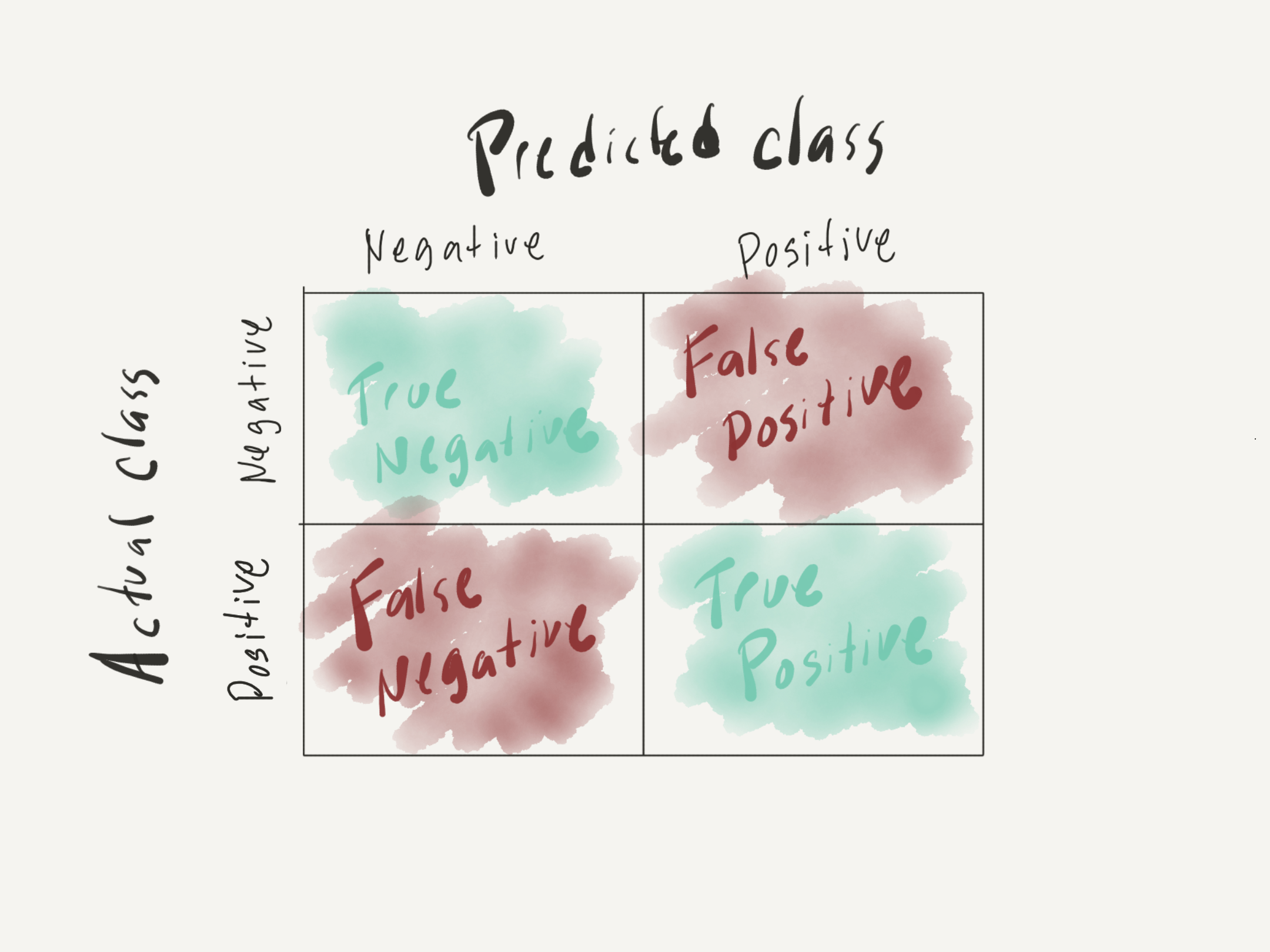
Figure 1: Confusion matrix

With this in mind we can use the tab_class confusion matrix to extract TP, TN, FP, and FN and create the calculations.

tab_class  # view confusion matrix

##             predicted_class
## actual_class  ham spam
##         ham  1161   40
##         spam    6  187

N <- sum(tab_class)  # sum of all predictions

TP <- tab_class[1, 1]  # positive, predicted positive
TN <- tab_class[2, 2]  # negative, predicted negative

FP <- tab_class[1, 2]  # negative, predicted positive
FN <- tab_class[2, 1]  # positive, predicted negative

# Summary statistics

accuracy <- (TP + TN)/N  # higher correct predictions (TP and TN) increase accuracy
precision <- TP/(TP + FP)  # lower FP increases precision
recall <- TP/(TP + FN)  # lower FN increases recall

f1_score <- 2 * ((precision * recall)/(precision + recall))

Production

Now, if we were satisfied with this model and wanted to put it into use to filter real SMS text messages, we could create a function to do just that.

We just need to include the step to tokenize the new messages in the same way we did to create the model and then create a dfm of these tokens as features. Then we match the features from the model and apply the model to the new message and report the class prediction as the result.

predict_sms_type <- function(sms_message, nb_model) {
  # Function
  # Takes a character vector of sms messages and provides
  # a prediction as to whether the message is spam or ham
  # given the given trained NB model
  
sms_tokens <- 
  tokens(x = sms_message, # character vector
         what = "word", # tokenize by words
         remove_punct = TRUE, # remove punctuation
         remove_numbers = FALSE) %>% # remove numbers
  tokens_tolower() # lowercase all characters

sms_dfm <- 
  dfm(sms_tokens) # create a document-frequency matrix
  
  # Match features from the Naive Bayes model
  dfm_matched <- 
    dfm_match(sms_dfm, features = featnames(nb_model$x))
  
  # Predict class for the given review
  predicted_class <- predict(nb_model, newdata = dfm_matched)
  
  as.character(predicted_class)
}


predict_sms_type(sms_message = "Hey how's it going?", nb_model = nb1)

## [1] "ham"

predict_sms_type(sms_message = "Call now to order this amazing product!!", nb_model = nb1)

## [1] "spam"

As you can see we can now create our own text messages and have them filtered by the algorithm that we have developed here.

Summary

In this Recipe, I demonstrated the steps involved in creating a text classification model. We then evaluated the training model and then applied it to the test data. The evaluation of both the training and testing predictions show that they were highly accurate. Since these results were very promising I demonstrated how we can turn a trained model into an actual spam filter.

Below I’ve included the code summary of the necessary steps to implement this prediction model.

# Get SMS dataset ---
sms_df <- tadr::sms # load dataset from tadr package

# Create corpus object ---
sms_corpus <- # quanteda corpus object
  corpus(sms_df, # data frame
         text_field = "message") # text field

sms_corpus$doc_id <- # create a new column `doc_id`
  1:ndoc(sms_corpus) # add numeric id to each text message

# Create tokens object
sms_tokens <- 
  tokens(x = sms_corpus, # corpus object
         what = "word", # tokenize by words
         remove_punct = TRUE, # remove punctuation
         remove_numbers = FALSE) %>% # remove numbers
  tokens_tolower() # lowercase all characters

# Create testing/ training splits
set.seed(300) # make reproducible

num_docs <- 
  sms_dfm %>% # dfm object
  ndoc() # get number of documents

train_size <- 
  (num_docs * .75) %>% # get size of sample
  round() # round to nearest whole number

train_ids <- sample(x = 1:num_docs, # population
                   size = train_size, # size of sample
                   replace = FALSE) # without replacement
sms_dfm_train <- 
  sms_dfm %>% # dfm object
  dfm_subset(doc_id %in% train_ids) # subset matching doc_id and train_ids

sms_dfm_test <- 
  sms_dfm %>% # dfm object
  dfm_subset(!doc_id %in% train_ids) # subset non-matching doc_id and train_ids

# Train the NB model
nb1 <- 
  textmodel_nb(x = sms_dfm_train, # document-feature matrix
               y = sms_dfm_train$sms_type) # class labels

# Test the NB model
dfm_matched <- 
  dfm_match(sms_dfm_test, # test dfm
            features = featnames(nb1$x)) # (left) join with trained model features

predicted_class <- 
  predict(nb1, # trained model
          newdata = dfm_matched) # classify test dataset

# Evaluate model performance
actual_class <- 
  dfm_matched$sms_type # get actual class labels

tab_class <- 
  table(actual_class, predicted_class) # cross-tabulate actual and predicted class labels

caret::confusionMatrix(tab_class, mode = "prec_recall") # model performance statistics

References

Almeida, Tiago A., and Jos’e María G’omez Hildago. 2011. “SMS Spam Collection.” SMS Spam Collection v. 1. https://www.dt.fee.unicamp.br/~tiago/smsspamcollection/.

Benoit, Kenneth, Kohei Watanabe, Haiyan Wang, Paul Nulty, Adam Obeng, Stefan Müller, Akitaka Matsuo, and William Lowe. 2022. Quanteda: Quantitative Analysis of Textual Data. https://quanteda.io.