5 Acquire data

INCOMPLETE DRAFT

The scariest moment is always just before you start.

―–Stephen King

The essential questions for this chapter are:

What are the most common strategies for acquiring corpus data?
What programmatic steps can we take to ensure the acquisition process is reproducible?
What is the importance of documenting data?

There are three main ways to acquire corpus data using R that I will introduce you to: downloads, APIs, and web scraping. In this chapter we will start by manual and programmatically downloading a corpus as it is the most straightforward process for the novice R programmer and typically incurs the least number of steps. Along the way I will introduce some key R coding concepts including control statements and custom functions. Next I will cover using R packages to interface with APIs, both open-access and authentication-based. APIs will require us to delve into more detail about R objects and custom functions. Finally acquiring data from the web via webscraping is the most idiosyncratic and involves both knowledge of the web, more sophisticated R skills, and often some clever hacking skills. I will start with a crash course on the structure of web documents (HTML) and then scale up to a real-world example. To round out the chapter we will cover the process of ensuring that our data is documented in such a way as to provide sufficient information to understand its key sampling characteristics and the source from which it was drawn.

5.1 Downloads

5.1.1 Manual

The first acquisition method I will cover here is inherently non-reproducible from the standpoint that the programming implementation cannot acquire the data based solely on running the project code itself. In other words, it requires manual intervention. Manual downloads are typical for data resources which are not openly accessible on the public facing web. These can be resources that require institutional or private licensing (Language Data Consortium, International Corpus of English, BYU Corpora, etc.), require authorization/ registration (The Language Archive, COW Corpora, etc.), and/ or are only accessible via resource search interfaces (Corpus of Spanish in Southern Arizona, Corpus Escrito del Español como L2 (CEDEL2), etc.).

Let’s work with the CEDEL2 corpus (Lozano, 2009) which provides a search interface and open access to the data through the search interface. The homepage can be seen in Figure 5.1.

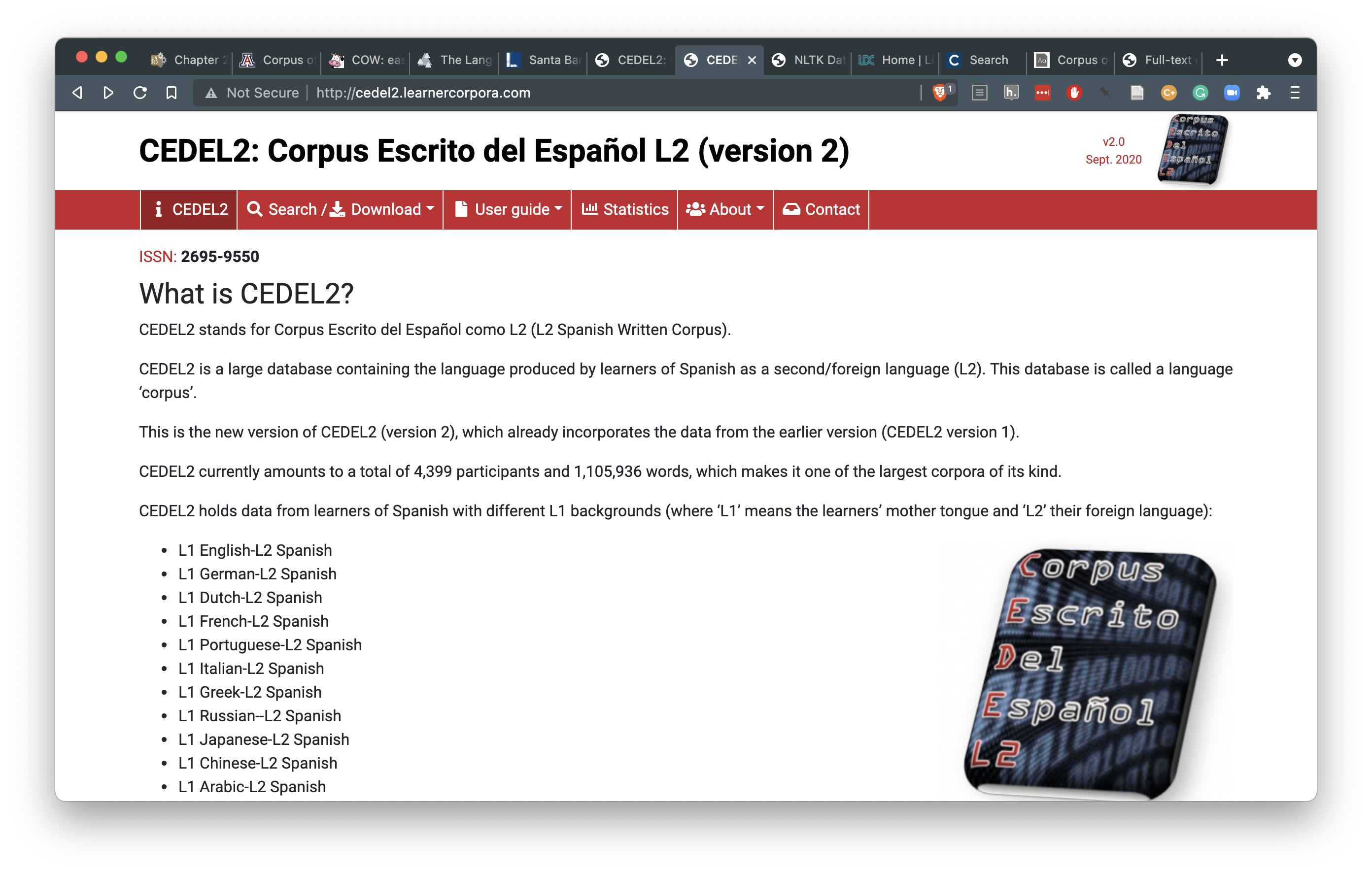
Figure 5.1: CEDEL2 Corpus homepage

Following the search/ download link you can find a search interface that allows the user to select the sub-corpus of interest. I’ve selected the subcorpus “Learners of L2 Spanish” and specified the L1 as English.

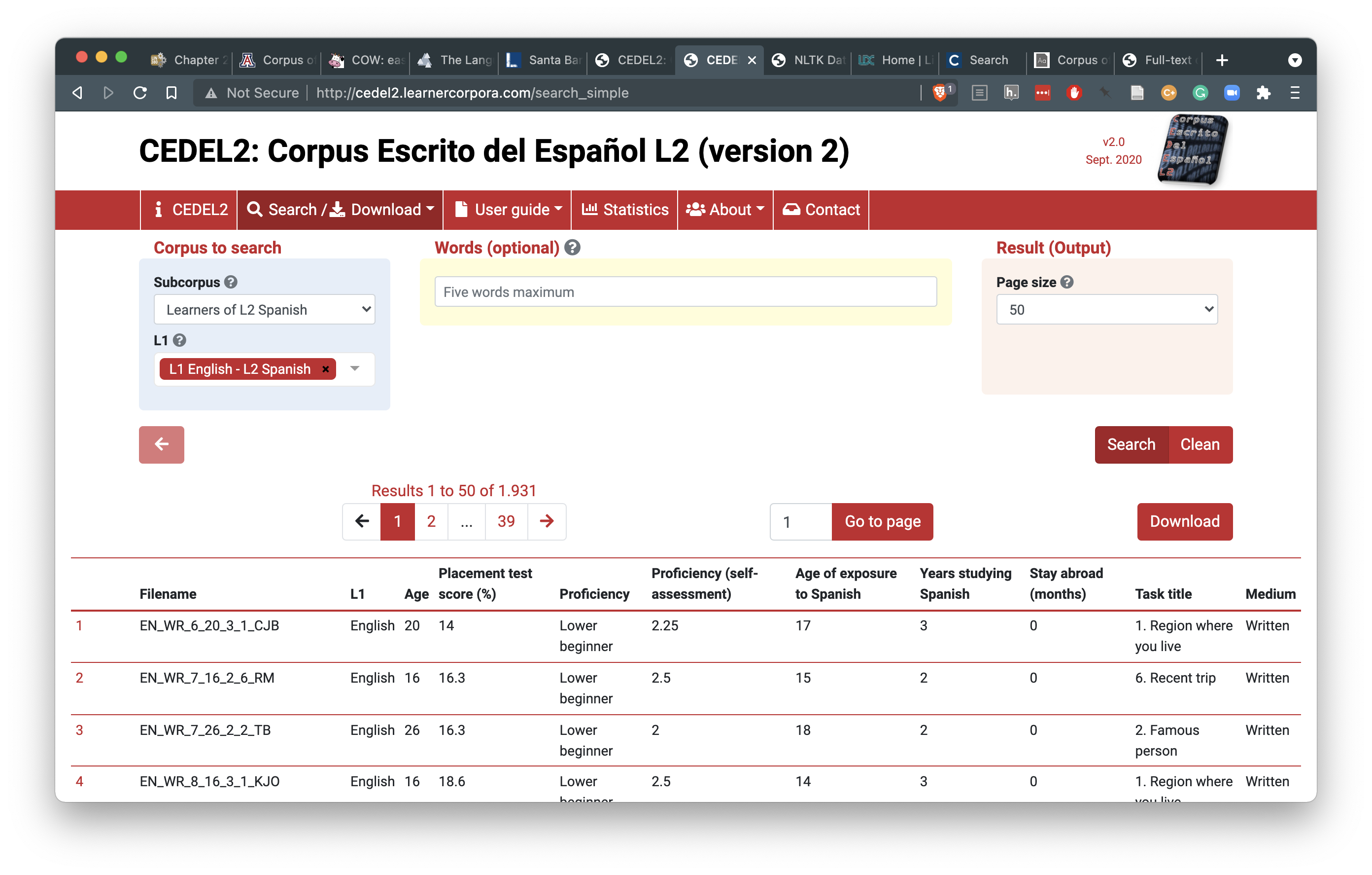
Figure 5.2: Search and download interface for the CEDEL2 Corpus

The ‘Download’ link now appears for this search criteria. Following this link will provide the user a form to fill out. This particular resource allows for access to different formats to download (Texts only, Texts with metadata, CSV (Excel), CSV (Others)). I will select the ‘CSV (Others)’ option so that the data is structured for easier processing downstream when we work to curate the data in our next processing step. Then I will choose to save the CSV in the data/original/ directory of my project and create a sub-directory called cedel2/.

data/
├── derived
└── original
    └── cedel2
       └── texts.csv

Other resources will inevitably include unique processes to obtaining the data, but in the end the data should be archived in the research structure in the data/original/ directory and be treated as ‘read-only’.

5.1.2 Programmatic

There are many resources that provide corpus data is directly accessible for which programmatic approaches can be applied. Let’s take a look at how this works starting with the a sample from the Switchboard Corpus, a corpus of 2,400 telephone conversations by 543 speakers. First we navigate to the site with a browser and download the file that we are looking for. In this case I found the Switchboard Corpus on the NLTK data repository site. More often than not this file will be some type of compressed archive file with an extension such as .zip or .tz, which is the case here. Archive files make downloading large single files or multiple files easy by grouping files and directories into one file. In R we can used the download.file() function from the base R library¹⁴. There are a number of arguments that a function may require or provide optionally. The download.file() function minimally requires two: url and destfile. That is the file to download and the location where it is to be saved to disk.

# Download .zip file and write to disk
download.file(url = "https://raw.githubusercontent.com/nltk/nltk_data/gh-pages/packages/corpora/switchboard.zip",
    destfile = "../data/original/switchboard.zip")

As we can see looking at the directory structure for data/ the switchboard.zip file has been downloaded.

data
├── derived
└── original
    └── switchboard.zip

Once an archive file is downloaded, however, the file needs to be ‘decompressed’ to reveal the file structure. To decompress this file we use the unzip() function with the arguments zipfile pointing to the .zip file and exdir specifying the directory where we want the files to be extracted to.

# Decompress .zip file and extract to our target directory
unzip(zipfile = "../data/original/switchboard.zip", exdir = "../data/original/")

The directory structure of data/ now should look like this:

data
├── derived
└── original
    ├── switchboard
    │   ├── README
    │   ├── discourse
    │   ├── disfluency
    │   ├── tagged
    │   ├── timed-transcript
    │   └── transcript
    └── switchboard.zip

At this point we have acquired the data programmatically and with this code as part of our workflow anyone could run this code and reproduce the same results. The code as it is, however, is not ideally efficient. Firstly the switchboard.zip file is not strictly needed after we decompress it and it occupies disk space if we keep it. And second, each time we run this code the file will be downloaded from the remote serve leading to unnecessary data transfer and server traffic. Let’s tackle each of these issues in turn.

To avoid writing the switchboard.zip file to disk (long-term) we can use the tempfile() function to open a temporary holding space for the file. This space can then be used to store the file, unzip it, and then the temporary file will be destroyed. We assign the temporary space to an R object we will name temp with the tempfile() function. This object can now be used as the value of the argument destfile in the download.file() function. Let’s also assign the web address to another object url which we will use as the value of the url argument.

# Create a temporary file space for our .zip file
temp <- tempfile()
# Assign our web address to `url`
url <- "https://raw.githubusercontent.com/nltk/nltk_data/gh-pages/packages/corpora/switchboard.zip"
# Download .zip file and write to disk
download.file(url, temp)

In the previous code I’ve used the values stored in the objects url and temp in the download.file() function without specifying the argument names –only providing the names of the objects. R will assume that values of a function map to the ordering of the arguments. If your values do not map to ordering of the arguments you are required to specify the argument name and the value. To view the ordering of objects hit TAB after entering the function name or consult the function documentation by prefixing the function name with ? and hitting ENTER.

At this point our downloaded file is stored temporarily on disk and can be accessed and decompressed to our target directory using temp as the value for the argument zipfile from the unzip() function. I’ve assigned our target directory path to target_dir and used it as the value for the argument exdir to prepare us for the next tweak on our approach.

# Assign our target directory to `target_dir`
target_dir <- "../data/original/"
# Decompress .zip file and extract to our target directory
unzip(zipfile = temp, exdir = target_dir)

Our directory structure now looks like this:

data
├── derived
└── original
    └── switchboard
        ├── README
        ├── discourse
        ├── disfluency
        ├── tagged
        ├── timed-transcript
        └── transcript

The second issue I raised concerns the fact that running this code as part of our project will repeat the download each time. Since we would like to be good citizens and avoid unnecessary traffic on the web it would be nice if our code checked to see if we already have the data on disk and if it exists, then skip the download, if not then download it.

To achieve this we need to introduce two new functions if() and dir.exists(). dir.exists() takes a path to a directory as an argument and returns the logical value, TRUE, if that directory exists, and FALSE if it does not. if() evaluates logical statements and processes subsequent code based on the logical value it is passed as an argument. Let’s look at a toy example.

num <- 1
if (num == 1) {
    cat(num, "is 1")
} else {
    cat(num, "is not 1")
}
#> 1 is 1

I assigned num to the value 1 and created a logical evaluation num == whose result is passed as the argument to if(). If the statement returns TRUE then the code withing the first set of curly braces {...} is run. If num == 1 is false, like in the code below, the code withing the braces following the else will be run.

num <- 2
if (num == 1) {
    cat(num, "is 1")
} else {
    cat(num, "is not 1")
}
#> 2 is not 1

The function if() is one of various functions that are called control statements. Theses functions provide a lot of power to make dynamic choices as code is run.

Before we get back to our key objective to avoid downloading resources that we already have on disk, let me introduce another strategy to making code more powerful and ultimately more efficient and as well as more legible –the custom function. Custom functions are functions that the user writes to create a set of procedures that can be run in similar contexts. I’ve created a custom function named eval_num() below.

eval_num <- function(num) {
    if (num == 1) {
        cat(num, "is 1")
    } else {
        cat(num, "is not 1")
    }
}

Let’s take a closer look at what’s going on here. The function function() creates a function in which the user decides what arguments are necessary for the code to perform its task. In this case the only necessary argument is the object to store a numeric value to be evaluated. I’ve called it num because it reflects the name of the object in our toy example, but there is nothing special about this name. It’s only important that the object names be consistently used. I’ve included our previous code (except for the hard-coded assignment of num) inside the curly braces and assigned the entire code chunk to eval_num.

We can now use the function eval_num() to perform the task of evaluating whether a value of num is or is not equal to 1.

eval_num(num = 1)
#> 1 is 1
eval_num(num = 2)
#> 2 is not 1
eval_num(num = 3)
#> 3 is not 1

I’ve put these coding strategies together with our previous code in a custom function I named get_zip_data(). There is a lot going on here. Take a look first and see if you can follow the logic involved given what you now know.

get_zip_data <- function(url, target_dir) {
    # Function: to download and decompress a .zip file to a target directory

    # Check to see if the data already exists if data does not exist, download/
    # decompress
    if (!dir.exists(target_dir)) {
        cat("Creating target data directory \n")  # print status message
        dir.create(path = target_dir, recursive = TRUE, showWarnings = FALSE)  # create target data directory
        cat("Downloading data... \n")  # print status message
        temp <- tempfile()  # create a temporary space for the file to be written to
        download.file(url = url, destfile = temp)  # download the data to the temp file
        unzip(zipfile = temp, exdir = target_dir, junkpaths = TRUE)  # decompress the temp file in the target directory
        cat("Data downloaded! \n")  # print status message
    } else {
        # if data exists, don't download it again
        cat("Data already exists \n")  # print status message
    }
}

OK. You should have recognized the general steps in this function: the argument url and target_dir specify where to get the data and where to write the decompressed files, the if() statement evaluates whether the data already exists, if not (!dir.exists(target_dir)) then the data is downloaded and decompressed, if it does exist (else) then it is not downloaded.

The prefixed ! in the logical expression dir.exists(target_dir) returns the opposite logical value. This is needed in this case so when the target directory exists, the expression will return FALSE, not TRUE, and therefore not proceed in downloading the resource.

There are a couple key tweaks I’ve added that provide some additional functionality. For one I’ve included the function dir.create() to create the target directory where the data will be written. I’ve also added an additional argument to the unzip() function, junkpaths = TRUE. Together these additions allow the user to create an arbitrary directory path where the files, and only the files, will be extracted to on our disk. This will discard the containing directory of the .zip file which can be helpful when we want to add multiple .zip files to the same target directory.

A practical scenario where this applies is when we want to download data from a corpus that is contained in multiple .zip files but still maintain these files in a single primary data directory. Take for example the Santa Barbara Corpus. This corpus resource includes a series of interviews in which there is one .zip file, SBCorpus.zip which contains the transcribed interviews and another .zip file, metadata.zip which organizes the meta-data associated with each speaker. Applying our initial strategy to download and decompress the data will lead to the following directory structure:

data
├── derived
└── original
    ├── SBCorpus
    │   ├── TRN
    │   └── __MACOSX
    │       └── TRN
    └── metadata
        └── __MACOSX

By applying our new custom function get_zip_data() to the transcriptions and then the meta-data we can better organize the data.

# Download corpus transcriptions
get_zip_data(url = "http://www.linguistics.ucsb.edu/sites/secure.lsit.ucsb.edu.ling.d7/files/sitefiles/research/SBC/SBCorpus.zip",
    target_dir = "../data/original/sbc/transcriptions/")

# Download corpus meta-data
get_zip_data(url = "http://www.linguistics.ucsb.edu/sites/secure.lsit.ucsb.edu.ling.d7/files/sitefiles/research/SBC/metadata.zip",
    target_dir = "../data/original/sbc/meta-data/")

data
├── derived
└── original
    └── sbc
        ├── meta-data
        └── transcriptions

If we add data from other sources we can keep them logical separate and allow our data collection to scale without creating unnecessary complexity. Let’s add the Switchboard Corpus sample using our get_zip_data() function to see this in action.

# Download corpus
get_zip_data(url = "https://raw.githubusercontent.com/nltk/nltk_data/gh-pages/packages/corpora/switchboard.zip",
    target_dir = "../data/original/scs/")

data
├── derived
└── original
    ├── sbc
    │   ├── meta-data
    │   └── transcriptions
    └── scs
        ├── README
        ├── discourse
        ├── disfluency
        ├── tagged
        ├── timed-transcript
        └── transcript

At this point we have what we need to continue to the next step in our data analysis project. But before we go, we should do some housekeeping to document and organize this process to make our work reproducible. We will take advantage of the project-template directory structure, seen below.

├── README.md
├── _pipeline.R
├── analysis
│   ├── 1_acquire_data.Rmd
│   ├── 2_curate_dataset.Rmd
│   ├── 3_transform_dataset.Rmd
│   ├── 4_analyze_dataset.Rmd
│   ├── 5_generate_article.Rmd
│   ├── _session-info.Rmd
│   ├── _site.yml
│   ├── index.Rmd
│   └── references.bib
├── data
│   ├── derived
│   └── original
│       ├── sbc
│       └── scs
├── functions
└── output
    ├── figures
    └── results

First it is good practice to separate custom functions from our processing scripts. We can create a file in our functions/ directory named acquire_functions.R and add our custom function get_zip_data() there.

Note that that the acquire_functions.R file is an R script, not an Rmarkdown document. Therefore code chunks that are used in .Rmd files are not used, only the R code itself.

We then use the source() function to read that function into our current script to make it available to use as needed. It is good practice to source your functions in the SETUP section of your script.

# Load custom functions for this project
source(file = "../functions/acquire_functions.R")

In this section, to sum up, we’ve covered how to access, download, and organize data contained in .zip files; the most common format for language data found on repositories and individual sites. This included an introduction to a few key R programming concepts and strategies including using functions, writing custom functions, and controlling program flow with control statements. Our approach was to gather data while also keeping in mind the reproducibility of the code. To this end I introduced programming strategies for avoiding unnecessary web traffic (downloads), scalable directory creation, and data documentation.

The custom function get_zip_data() works with .zip files. There are many other compressed file formats (e.g. .gz, .tar, .tgz), however. In the R package tadr that accompanies this coursebook, a modified version of the get_zip_data() function, get_compressed_data(), extends the same logic to deal with a wider range of compressed file formats, including .zip files.

Explore this function’s documentation (?tadr::get_compressed_data()) and/ or view the code (tadr::get_compressed_data) to better understand this function.

5.2 APIs

A convenient alternative method for acquiring data in R is through package interfaces to web services. These interfaces are built using R code to make connections with resources on the web through Application Programming Interfaces (APIs). Websites such as Project Gutenberg, Twitter, Facebook, and many others provide APIs to allow access to their data under certain conditions, some more limiting for data collection than others. Programmers (like you!) in the R community take up the task of wrapping calls to an API with R code to make accessing that data from R possible. For example, gutenbergr provides access to Project Gutenberg, rtweet to Twitter, and Rfacebook to Facebook.¹⁵

5.2.1 Open access

Using R package interfaces, however, often requires some more knowledge about R objects and functions. Let’s take a look at how to access data from Project Gutenberg through the gutenbergr package. Along the way we will touch upon various functions and concepts that are key to working with the R data types vectors and data frames including filtering and writing tabular data to disk in plain-text format.

To get started let’s install and/ or load the gutenbergr package. If a package is not part of the R base library, we cannot assume that the user will have the package in their library. The standard approach for installing and then loading a package is by using the install.packages() function and then calling library().

install.packages("gutenbergr")  # install `gutenbergr` package
library(gutenbergr)  # load the `gutenbergr` package

This approach works just fine, but luck has it that there is an R package for installing and loading packages! The pacman package includes a set of functions for managing packages. A very useful one is p_load() which will look for a package on a system, load it if it is found, and install and then load it if it is not found. This helps potentially avoid using unnecessary bandwidth to install packages that may already exist on a user’s system. But, to use pacman we need to include the code to install and load it with the functions install.packages() and library(). I’ve included some code that will mimic the behavior of p_load() for installing pacman itself, but as you can see it is not elegant, luckily it’s only used once as we add it to the SETUP section of our master file, _pipeline.R.

# Load `pacman`. If not installed, install then load.
if (!require("pacman", character.only = TRUE)) {
    install.packages("pacman")
    library("pacman", character.only = TRUE)
}

Now that we have pacman installed and loaded into our R session, let’s use the p_load() function to make sure to install/ load the two packages we will need for the upcoming tasks. If you are following along with the project_template, add this code within the SETUP section of the 1_acquire_data.Rmd file.

# Script-specific options or packages
pacman::p_load(tidyverse, gutenbergr)

Note that the arguments tidyverse and gutenbergr are comma-separated but not quoted when using p_load(). When using install.packages() to install, package names need to be quoted (character strings). library() can take quotes or no quotes, but only one package at a time.

Project Gutenberg provides access to thousands of texts in the public domain. The gutenbergr package contains a set of tables, or data frames in R speak, that index the meta-data for these texts broken down by text (gutenberg_metadata), author (gutenberg_authors), and subject (gutenberg_subjects). I’ll use the glimpse() function loaded in the tidyverse package ¹⁶ to summarize the structure of these data frames.

glimpse(gutenberg_metadata)  # summarize text meta-data
#> Rows: 51,997
#> Columns: 8
#> $ gutenberg_id        <int> 0, 1, 2, 3, 4, 5, 6, 7, 8, 9, 10, 11, 12, 13, 14, …
#> $ title               <chr> NA, "The Declaration of Independence of the United…
#> $ author              <chr> NA, "Jefferson, Thomas", "United States", "Kennedy…
#> $ gutenberg_author_id <int> NA, 1638, 1, 1666, 3, 1, 4, NA, 3, 3, NA, 7, 7, 7,…
#> $ language            <chr> "en", "en", "en", "en", "en", "en", "en", "en", "e…
#> $ gutenberg_bookshelf <chr> NA, "United States Law/American Revolutionary War/…
#> $ rights              <chr> "Public domain in the USA.", "Public domain in the…
#> $ has_text            <lgl> TRUE, TRUE, TRUE, TRUE, TRUE, TRUE, TRUE, TRUE, TR…
glimpse(gutenberg_authors)  # summarize authors meta-data
#> Rows: 16,236
#> Columns: 7
#> $ gutenberg_author_id <int> 1, 3, 4, 5, 7, 8, 9, 10, 12, 14, 16, 17, 18, 20, 2…
#> $ author              <chr> "United States", "Lincoln, Abraham", "Henry, Patri…
#> $ alias               <chr> NA, NA, NA, NA, "Dodgson, Charles Lutwidge", NA, "…
#> $ birthdate           <int> NA, 1809, 1736, NA, 1832, NA, 1819, 1860, 1805, 17…
#> $ deathdate           <int> NA, 1865, 1799, NA, 1898, NA, 1891, 1937, 1844, 18…
#> $ wikipedia           <chr> NA, "http://en.wikipedia.org/wiki/Abraham_Lincoln"…
#> $ aliases             <chr> NA, "United States President (1861-1865)/Lincoln, …
glimpse(gutenberg_subjects)  # summarize subjects meta-data
#> Rows: 140,173
#> Columns: 3
#> $ gutenberg_id <int> 1, 1, 1, 1, 2, 2, 2, 2, 3, 3, 3, 4, 4, 4, 4, 5, 5, 5, 5, …
#> $ subject_type <chr> "lcc", "lcsh", "lcsh", "lcc", "lcc", "lcsh", "lcsh", "lcc…
#> $ subject      <chr> "E201", "United States. Declaration of Independence", "Un…

The gutenberg_metadata, gutenberg_authors, and gutenberg_subjects are periodically updated. To check to see when each data frame was last updated run:

attr(gutenberg_metadata, "date_updated")

To download the text itself we use the gutenberg_download() function which takes one required argument, gutenberg_id. The gutenberg_download() function is what is known as ‘vectorized’, that is, it can take a single value or multiple values for the argument gutenberg_id. Vectorization refers to the process of applying a function to each of the elements stored in a vector –a primary object type in R. A vector is a grouping of values of one of various types including character (chr), integer (int), double (dbl), and logical (lgl) and a data frame is a grouping of vectors. The gutenberg_download() function takes an integer vector which can be manually added or selected from the gutenberg_metadata or gutenberg_subjects data frames using the $ operator (e.g. gutenberg_metadata$gutenberg_id).

Let’s first add them manually here as a toy example by generating a vector of integers from 1 to 5 assigned to the variable name ids.

ids <- 1:5  # integer vector of values 1 to 5
ids
#> [1] 1 2 3 4 5

To download the works from Project Gutenberg corresponding to the gutenberg_ids 1 to 5, we pass the ids object to the gutenberg_download() function.

works_sample <- gutenberg_download(gutenberg_id = ids)  # download works with `gutenberg_id` 1-5
glimpse(works_sample)  # summarize `works` dataset
#> Rows: 2,959
#> Columns: 2
#> $ gutenberg_id <int> 1, 1, 1, 1, 1, 1, 1, 1, 1, 1, 1, 1, 1, 1, 1, 1, 1, 1, 1, …
#> $ text         <chr> "December, 1971  [Etext #1]", "", "", "The Project Gutenb…

Two attributes are returned: gutenberg_id and text. The text column contains values for each line of text (delimited by a carriage return) for each of the 5 works we downloaded. There are many more attributes available from the Project Gutenberg API that can be accessed by passing a character vector of the attribute names to the argument meta_fields. The column names of the gutenberg_metadata data frame contains the available attributes.

names(gutenberg_metadata)  # print the column names of the `gutenberg_metadata` data frame
#> [1] "gutenberg_id"        "title"               "author"             
#> [4] "gutenberg_author_id" "language"            "gutenberg_bookshelf"
#> [7] "rights"              "has_text"

Let’s augment our previous download with the title and author of each of the works. To create a character vector we use the c() function, then, quote and delimit the individual elements of the vector with a comma.

# download works with `gutenberg_id` 1-5 including `title` and `author` as
# attributes
works_sample <- gutenberg_download(gutenberg_id = ids, meta_fields = c("title", "author"))
glimpse(works_sample)  # summarize dataset
#> Rows: 2,959
#> Columns: 4
#> $ gutenberg_id <int> 1, 1, 1, 1, 1, 1, 1, 1, 1, 1, 1, 1, 1, 1, 1, 1, 1, 1, 1, …
#> $ text         <chr> "December, 1971  [Etext #1]", "", "", "The Project Gutenb…
#> $ title        <chr> "The Declaration of Independence of the United States of …
#> $ author       <chr> "Jefferson, Thomas", "Jefferson, Thomas", "Jefferson, Tho…

Now, in a more practical scenario we would like to select the values of gutenberg_id by some principled query such as works from a specific author, language, or subject. To do this we first query either the gutenberg_metadata data frame or the gutenberg_subjects data frame. Let’s say we want to download a random sample of 10 works from English Literature (Library of Congress Classification, “PR”). Using the dplyr::filter() function (dplyr is part of the tidyverse package set) we first extract all the Gutenberg ids from gutenberg_subjects where subject_type == "lcc" and subject == "PR" assigning the result to ids.¹⁷

# filter for only English literature
ids <- filter(gutenberg_subjects, subject_type == "lcc", subject == "PR")
glimpse(ids)
#> Rows: 7,100
#> Columns: 3
#> $ gutenberg_id <int> 11, 12, 13, 16, 20, 26, 27, 35, 36, 42, 43, 46, 58, 60, 8…
#> $ subject_type <chr> "lcc", "lcc", "lcc", "lcc", "lcc", "lcc", "lcc", "lcc", "…
#> $ subject      <chr> "PR", "PR", "PR", "PR", "PR", "PR", "PR", "PR", "PR", "PR…

The operators = and == are not equivalents. == is used for logical evaluation and = is an alternate notation for variable assignment (<-).

The gutenberg_subjects data frame does not contain information as to whether a gutenberg_id is associated with a plain-text version. To limit our query to only those English Literature works with text, we filter the gutenberg_metadata data frame by the ids we have selected in ids and the attribute has_text in the gutenberg_metadata data frame.

# Filter for only those works that have text
ids_has_text <- 
  filter(gutenberg_metadata, 
         gutenberg_id %in% ids$gutenberg_id, 
         has_text == TRUE)
glimpse(ids_has_text)
#> Rows: 6,724
#> Columns: 8
#> $ gutenberg_id        <int> 11, 12, 13, 16, 20, 26, 27, 35, 36, 42, 43, 46, 58…
#> $ title               <chr> "Alice's Adventures in Wonderland", "Through the L…
#> $ author              <chr> "Carroll, Lewis", "Carroll, Lewis", "Carroll, Lewi…
#> $ gutenberg_author_id <int> 7, 7, 7, 10, 17, 17, 23, 30, 30, 35, 35, 37, 17, 4…
#> $ language            <chr> "en", "en", "en", "en", "en", "en", "en", "en", "e…
#> $ gutenberg_bookshelf <chr> "Children's Literature", "Children's Literature/Be…
#> $ rights              <chr> "Public domain in the USA.", "Public domain in the…
#> $ has_text            <lgl> TRUE, TRUE, TRUE, TRUE, TRUE, TRUE, TRUE, TRUE, TR…

A couple R programming notes on the code phrase gutenberg_id %in% ids$gutenberg_id. First, the $ symbol in ids$gutenberg_id is the programmatic way to target a particular column in an R data frame. In this example we select the ids data frame and the column gutenberg_id, which is a integer vector. The gutenberg_id variable that precedes the %in% operator does not need an explicit reference to a data frame because the primary argument of the filter() function is this data frame (gutenberg_metadata). Second, the %in% operator logically evaluates whether the vector elements in gutenberg_metadata$gutenberg_ids are also found in the vector ids$gutenberg_id returning TRUE and FALSE accordingly. This effectively filters those ids which are not in both vectors.

As we can see the number of works with text is fewer than the number of works listed, 7100 versus 6724. Now we can safely do our random selection of 10 works, with the function slice_sample() and be confident that the ids we select will contain text when we take the next step by downloading the data.

set.seed(123)  # make the sampling reproducible
ids_sample <- slice_sample(ids_has_text, n = 10)  # sample 10 works
glimpse(ids_sample)  # summarize the dataset
#> Rows: 10
#> Columns: 8
#> $ gutenberg_id        <int> 10564, 10784, 9316, 1540, 24450, 13821, 7595, 3818…
#> $ title               <chr> "Fairy Gold\nShip's Company, Part 4.", "Sentence D…
#> $ author              <chr> "Jacobs, W. W. (William Wymark)", "Jacobs, W. W. (…
#> $ gutenberg_author_id <int> 1865, 1865, 2364, 65, 999, 2685, 761, 1317, 3564, …
#> $ language            <chr> "en", "en", "en", "en", "en", "en", "en", "en", "e…
#> $ gutenberg_bookshelf <chr> NA, NA, NA, NA, "Adventure", "Fantasy", NA, NA, NA…
#> $ rights              <chr> "Public domain in the USA.", "Public domain in the…
#> $ has_text            <lgl> TRUE, TRUE, TRUE, TRUE, TRUE, TRUE, TRUE, TRUE, TR…

works_pr <- gutenberg_download(gutenberg_id = ids_sample$gutenberg_id, meta_fields = c("author",
    "title"))
glimpse(works_pr)  # summarize the dataset
#> Rows: 47,515
#> Columns: 4
#> $ gutenberg_id <int> 1540, 1540, 1540, 1540, 1540, 1540, 1540, 1540, 1540, 154…
#> $ text         <chr> "cover ", "", "", "", "THE TEMPEST", "", "", "", "by Will…
#> $ author       <chr> "Shakespeare, William", "Shakespeare, William", "Shakespe…
#> $ title        <chr> "The Tempest", "The Tempest", "The Tempest", "The Tempest…

At this point we have data and could move on to processing this dataset in preparation for analysis. However, we are aiming for a reproducible workflow and this code does not conform to our principle of modularity: each subsequent step in our analysis will depend on running this code first. Furthermore, running this code as it is creates issues with bandwidth, as in our previous examples from direct downloads. To address modularity we will write the dataset to disk in plain-text format. In this way each subsequent step in our analysis can access the dataset locally. To address bandwidth concerns, we will devise a method for checking to see if the dataset is already downloaded and skip the download, if possible, to avoid accessing the Project Gutenberg server unnecessarily.

To write our data frame to disk we will export it into a standard plain-text format for two-dimensional datasets: a CSV file (comma-separated value). The CSV structure for this dataset will look like this:

works_pr %>%
    head() %>%
    format_csv() %>%
    cat()
#> gutenberg_id,text,author,title
#> 1540,cover ,"Shakespeare, William",The Tempest
#> 1540,,"Shakespeare, William",The Tempest
#> 1540,,"Shakespeare, William",The Tempest
#> 1540,,"Shakespeare, William",The Tempest
#> 1540,THE TEMPEST,"Shakespeare, William",The Tempest
#> 1540,,"Shakespeare, William",The Tempest

The first line contains the names of the columns and subsequent lines the observations. Data points that contain commas themselves (e.g. “Shaw, Bernard”) are quoted to avoid misinterpreting these commas a deliminators in our data. To write this dataset to disk we will use the reader::write_csv() function.

write_csv(works_pr, file = "../data/original/gutenberg_works_pr.csv")

To avoid downloading dataset that already resides on disk, let’s implement a similar strategy to the one used for direct downloads (get_zip_data()). I’ve incorporated the code for sampling and downloading data for a particular subject from Project Gutenberg with a control statement to check if the dataset file already exists into a function I named get_gutenberg_subject(). Take a look at this function below.

get_gutenberg_subject <- function(subject, target_file, sample_size = 10) {
  # Function: to download texts from Project Gutenberg with 
  # a specific LCC subject and write the data to disk.
  
  pacman::p_load(tidyverse, gutenbergr) # install/load necessary packages
  
  # Check to see if the data already exists
  if(!file.exists(target_file)) { # if data does not exist, download and write
    target_dir <- dirname(target_file) # generate target directory for the .csv file
    dir.create(path = target_dir, recursive = TRUE, showWarnings = FALSE) # create target data directory
    cat("Downloading data... \n") # print status message
    # Select all records with a particular LCC subject
    ids <- 
      filter(gutenberg_subjects, 
             subject_type == "lcc", subject == subject) # select subject
    # Select only those records with plain text available
    set.seed(123) # make the sampling reproducible
    ids_sample <- 
      filter(gutenberg_metadata, 
             gutenberg_id %in% ids$gutenberg_id, # select ids in both data frames 
             has_text == TRUE) %>% # select those ids that have text
      slice_sample(n = sample_size) # sample N works 
    # Download sample with associated `author` and `title` metadata
    works_sample <- 
      gutenberg_download(gutenberg_id = ids_sample$gutenberg_id, 
                         meta_fields = c("author", "title"))
    # Write the dataset to disk in .csv format
    write_csv(works_sample, file = target_file)
    cat("Data downloaded! \n") # print status message
  } else { # if data exists, don't download it again
    cat("Data already exists \n") # print status message
  }
}

Adding this function to our function script functions/acquire_functions.R, we can now source this function in our analysis/1_acquire_data.Rmd script to download multiple subjects and store them in on disk in their own file.

Let’s download American Literature now (LCC code “PQ”).

# Download Project Gutenberg text for subject 'PQ' (American Literature) and
# then write this dataset to disk in .csv format
get_gutenberg_subject(subject = "PQ", target_file = "../data/original/gutenberg/works_pq.csv")

Applying this function to both the English and American Literature datasets, our data directory structure now looks like this:

data
├── derived
└── original
    ├── gutenberg
    │   ├── works_pq.csv
    │   └── works_pr.csv
    ├── sbc
    │   ├── meta-data
    │   └── transcriptions
    └── scs
        ├── README
        ├── discourse
        ├── disfluency
        ├── documentation
        ├── tagged
        ├── timed-transcript
        └── transcript

5.2.2 Authentication

Some APIs and the R interfaces that provide access to them require authentication. This may either be through an interactive process that is mediated between R and the web service and/ or by visiting the developer website of the particular API. In either case, there is an extra step that is necessary to make the connect to the API to access the data.

Let’s take a look at the popular micro-blogging platform Twitter. The rtweet package (Kearney, 2020) provides access to tweets in various ways. To get started install and/or load the rtweet package.

pacman::p_load(rtweet)  # install/load rtweet package

Now before a researcher can access data from Twitter with rtweet, an authentication token must be setup and made accessible. After following the steps for setting up an authentication token and saving it, that token can be accessed with the auth_as() function.

auth_as(twitter_auth)  # load the saved `twitter_auth` token

Now that we the R session is authenticated, we can explore a popular method for querying the Twitter API which searchs tweets (search_tweets) posted in the recent past (6-9 days).

Let’s look at a typical query using the search_tweets() function.

rt_latinx <- 
  search_tweets(q = "latinx", # query term
                n = 100, # number of tweets desired
                type = "mixed", # a mix of `recent` and `popular` tweets
                include_rts = FALSE) # do not include RTs

Looking at the arguments in this function, we see I’ve specified the query term to be ‘latinx’. This is a single word query but if the query included multiple words, the spaces between would be interpreted as the logical AND (only match tweets with all the individual terms). If one would like to include multi-word expressions, the expressions should be enclosed by single quotes (i.e. q = "'spanish speakers' AND latinx"). Another approach would be to include the logical OR (match tweets with either of the terms). Multi-word expressions can be included as in the previous case. Of note, hashtags are acceptable terms, so q = "#latinx" would match tweets with this hashtag.

The number of results has been set at ‘100’, but this is the default, so I could have left it out. But you can increase the number of desired tweets. There are rate limits which cap the number of tweets you can access in a given 15-minute time period.

Another argument of importance is the type argument. This argument has three possible attributes popular, recent, and mixed. When the popular attribute he Twitter API will tend to return fewer tweets than specified by n. With recent or mixed you will most likely get the n you specified (note that mixed is a mix of popular and recent).

A final argument to note is the include_rts whose attribute is logical. If FALSE no retweets will be included in the results. This is often what a language researcher will want.

Now, once the search_tweets query has been run, there a a large number of variables that are included in the resulting data frame. Here’s an overview of the names of the variables and the vector types for each variable.

Table 5.1: Variables and variable types returned from Twitter API via rtweet’s `search_tweets()` function.
created_at	character
id	double
id_str	character
full_text	character
truncated	logical
display_text_range	double
entities	list
metadata	list
source	character
in_reply_to_status_id	double
in_reply_to_status_id_str	character
in_reply_to_user_id	double
in_reply_to_user_id_str	character
in_reply_to_screen_name	character
geo	logical
coordinates	list
place	list
contributors	logical
is_quote_status	logical
retweet_count	integer
favorite_count	integer
favorited	logical
retweeted	logical
lang	character
possibly_sensitive	logical
quoted_status_id	double
quoted_status_id_str	character
quoted_status	list
text	character
favorited_by	logical
display_text_width	logical
retweeted_status	logical
quoted_status_permalink	logical
query	logical
possibly_sensitive_appealable	logical

The Twitter API documentation for the standard Search Tweets call, which is what search_tweets() interfaces with has quite a few variables (35 to be exact). For many purposes it is not necessary to keep all the variables. Furthermore, since we will want to write a plain-text file to disk as part of our project, we will need to either convert or eliminate any of the variables that are marked as type list. The most common variable to convert is the coordinates variable, as it will contain the geolocation codes for those Twitter users’ tweets captured in the query that have geolocation enabled on their device. It is of note, however, that using search_tweets() without specifying that only tweets with geocodes should be captured (geocode =) will tend to return very few, if any, tweets with geolocation information as the majority of Twitter users do not have geolocation enabled.

Let’s assume that we want to keep all the variables that are not of type list. One option is to use select() and name each variable we want to keep. On the other hand we can use a combination of select() and negated !where() to select all the variables that are not lists (is_list). Let’s do the later approach.

rt_latinx_subset <- 
  rt_latinx %>% # dataset
  select(!where(is_list))  # select all variables that are NOT lists

rt_latinx_subset %>% # subsetted dataset
  glimpse() # overview
#> Rows: 100
#> Columns: 30
#> $ created_at                    <chr> "Sun Sep 26 17:38:06 +0000 2021", "Sun S…
#> $ id                            <dbl> 1.44e+18, 1.44e+18, 1.44e+18, 1.44e+18, …
#> $ id_str                        <chr> "1442181701967302659", "1442196629801488…
#> $ full_text                     <chr> "If we call it Latinx Mass they can't ca…
#> $ truncated                     <lgl> FALSE, FALSE, FALSE, FALSE, FALSE, FALSE…
#> $ display_text_range            <dbl> 57, 177, 166, 23, 261, 153, 202, 211, 57…
#> $ source                        <chr> "<a href=\"https://mobile.twitter.com\" …
#> $ in_reply_to_status_id         <dbl> NA, NA, NA, 1.44e+18, NA, NA, NA, NA, 1.…
#> $ in_reply_to_status_id_str     <chr> NA, NA, NA, "1437436224042635269", NA, N…
#> $ in_reply_to_user_id           <dbl> NA, NA, NA, 4.26e+08, NA, NA, NA, NA, 2.…
#> $ in_reply_to_user_id_str       <chr> NA, NA, NA, "426159377", NA, NA, NA, NA,…
#> $ in_reply_to_screen_name       <chr> NA, NA, NA, "MorganStanley", NA, NA, NA,…
#> $ geo                           <lgl> NA, NA, NA, NA, NA, NA, NA, NA, NA, NA, …
#> $ contributors                  <lgl> NA, NA, NA, NA, NA, NA, NA, NA, NA, NA, …
#> $ is_quote_status               <lgl> FALSE, FALSE, FALSE, FALSE, TRUE, FALSE,…
#> $ retweet_count                 <int> 351, 124, 62, 0, 0, 0, 0, 0, 0, 0, 0, 1,…
#> $ favorite_count                <int> 3902, 898, 280, 0, 0, 0, 0, 0, 0, 7, 0, …
#> $ favorited                     <lgl> FALSE, FALSE, FALSE, FALSE, FALSE, FALSE…
#> $ retweeted                     <lgl> FALSE, FALSE, FALSE, FALSE, FALSE, FALSE…
#> $ lang                          <chr> "en", "en", "es", "en", "en", "en", "en"…
#> $ possibly_sensitive            <lgl> NA, FALSE, FALSE, FALSE, FALSE, FALSE, F…
#> $ quoted_status_id              <dbl> NA, NA, NA, NA, 1.44e+18, NA, NA, NA, NA…
#> $ quoted_status_id_str          <chr> NA, NA, NA, NA, "1442475408058830856", N…
#> $ text                          <chr> "If we call it Latinx Mass they can't ca…
#> $ favorited_by                  <lgl> NA, NA, NA, NA, NA, NA, NA, NA, NA, NA, …
#> $ display_text_width            <lgl> NA, NA, NA, NA, NA, NA, NA, NA, NA, NA, …
#> $ retweeted_status              <lgl> NA, NA, NA, NA, NA, NA, NA, NA, NA, NA, …
#> $ quoted_status_permalink       <lgl> NA, NA, NA, NA, NA, NA, NA, NA, NA, NA, …
#> $ query                         <lgl> NA, NA, NA, NA, NA, NA, NA, NA, NA, NA, …
#> $ possibly_sensitive_appealable <lgl> NA, NA, NA, NA, NA, NA, NA, NA, NA, NA, …

Now we have the 30 variables which can be written to disk as a plain-text file. Let’s go ahead a do this, but wrap it in a function that does all the work we’ve just laid out in one function. In addition we will check to see if the same query has been run, and skip running the query if the dataset is on disk.

write_search_tweets <- 
  function(query, path, n = 100, type = "mixed", include_rts = FALSE) {
    # Function
    # Conduct a Twitter search query and write the results to a csv file
    
    if(!file.exists(path)) { # check to see if the file already exists
      cat("File does not exist \n") # message
      
      library(rtweet) # to use Twitter API
      library(tidyverse) # to manipulate data
      
      auth_get() # get authentication token
      
      results <- # query results
        search_tweets(q = query, # query term
                      n = n, # number of tweets desired (default 100)
                      type = type, # type of query
                      include_rts = include_rts) %>%  # to include RTs
        select(!where(is_list))  # remove list variables
      
      if(!dir.exists(dirname(path))) { # isolate directory and check if exists
        cat("Creating directory \n") # message
        
        dir.create(path = dirname(path), # isolate and create directory (remove file name)
                   recursive = TRUE, # create embedded directories if necessary
                   showWarnings = FALSE) # do not report warnings
      }
      
      write_csv(x = results, file = path) # write results to csv file 
      cat("Twitter search results written to disk \n") # message
      
    } else {
      cat("File already exists! \n") # message
    }
  }

Let’s run this function with the same query as above.

write_search_tweets(query = "latinx", path = "../data/original/twitter/rt_latinx.csv")

And the appropriate directory structure and file have been written to disk.

data/original/twitter/
└── rt_latinx.csv

In sum, this subsection provided an overview to acquiring data from web service APIs through R packages. We took at closer look at the gutenbergr package which provides programmatic access to works available on Project Gutenberg and the rtweet package which provides authenticated access to Twitter. Working with package interfaces requires more knowledge of R including loading/ installing packages, working with vectors and data frames, and exporting data from an R session. We touched on these programming concepts and also outlined a method to create a reproducible workflow.

5.3 Web scraping

There are many resources available through manula and direct downloads from repositories and individual sites and R package interfaces to web resources with APIs, but these resources are relatively limited to the amount of public-facing textual data recorded on the web. In the case that you want to acquire data from webpages, R can be used to access the web programmatically through a process known as web scraping. The complexity of web scrapes can vary but in general it requires more advanced knowledge of R as well as the structure of the language of the web: HTML (Hypertext Markup Language).

5.3.1 A toy example

HTML is a cousin of XML (eXtensible Markup Language) and as such organizes web documents in a hierarchical format that is read by your browser as you navigate the web. Take for example the toy webpage I created as a demonstration in Figure 5.3.

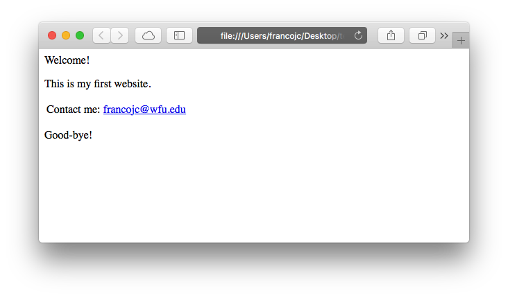
Figure 5.3: Example web page.

The file accessed by my browser to render this webpage is test.html and in plain-text format looks like this:


<html>
  <head>
    <title>My website</title>
  </head>
  <body>
    <div class="intro">
      <p>Welcome!</p>
      <p>This is my first website. </p>
    </div>
    <table>
      <tr>
        <td>Contact me:</td>
        <td>
          <a href="mailto:francojc@wfu.edu">francojc@wfu.edu</a>
        </td>
      </tr>
    </table>
    <div class="conc">
      <p>Good-bye!</p>
    </div>
  </body>
</html>

Each element in this file is delineated by an opening and closing tag, <head></head>. Tags are nested within other tags to create the structural hierarchy. Tags can take class and id labels to distinguish them from other tags and often contain other attributes that dictate how the tag is to behave when rendered visually by a browser. For example, there are two <div> tags in our toy example: one has the label class = "intro" and the other class = "conc". <div> tags are often used to separate sections of a webpage that may require special visual formatting. The <a> tag, on the other hand, creates a web link. As part of this tag’s function, it requires the attribute href= and a web protocol –in this case it is a link to an email address mailto:francojc@wfu.edu. More often than not, however, the href= contains a URL (Uniform Resource Locator). A working example might look like this: <a href="https://francojc.github.io/">My homepage</a>.

The aim of a web scrape is to download the HTML file, parse the document structure, and extract the elements containing the relevant information we wish to capture. Let’s attempt to extract some information from our toy example. To do this we will need the rvest(Wickham, 2021) package. First, install/load the package, then, read and parse the HTML from the character vector named web_file assigning the result to html.

pacman::p_load(rvest)  # install/ load `rvest`

html <- read_html(web_file)  # read raw html and parse to xml
html
#> {html_document}
#> <html>
#> [1] <head>\n<meta http-equiv="Content-Type" content="text/html; charset=UTF-8 ...
#> [2] <body>\n    <div class="intro">\n      <p>Welcome!</p>\n      <p>This is  ...

read_html() parses the raw HTML into an object of class xml_document. The summary output above shows that tags the HTML structure have been parsed into ‘elements’. The tag elements can be accessed by using the html_elements() function by specifying the tag to isolate.

html %>%
    html_elements("div")
#> {xml_nodeset (2)}
#> [1] <div class="intro">\n      <p>Welcome!</p>\n      <p>This is my first web ...
#> [2] <div class="conc">\n      <p>Good-bye!</p>\n    </div>

Notice that html_elements("div") has returned both div tags. To isolate one of tags by its class, we add the class name to the tag separating it with a ..

html %>%
    html_elements("div.intro")
#> {xml_nodeset (1)}
#> [1] <div class="intro">\n      <p>Welcome!</p>\n      <p>This is my first web ...

Great. Now say we want to drill down and isolate the subordinate <p> nodes. We can add p to our node filter.

html %>%
    html_elements("div.intro p")
#> {xml_nodeset (2)}
#> [1] <p>Welcome!</p>
#> [2] <p>This is my first website. </p>

To extract the text contained within a node we use the html_text() function.

html %>%
    html_elements("div.intro p") %>%
    html_text()
#> [1] "Welcome!"                   "This is my first website. "

The result is a character vector with two elements corresponding to the text contained in each <p> tag. If you were paying close attention you might have noticed that the second element in our vector includes extra whitespace after the period. To trim leading and trailing whitespace from text we can add the trim = TRUE argument to html_text().

html %>%
    html_elements("div.intro p") %>%
    html_text(trim = TRUE)
#> [1] "Welcome!"                  "This is my first website."

From here we would then work to organize the text into a format we want to store it in and write the results to disk. Let’s leave writing data to disk for later in the chapter. For now keep our focus on working with rvest to acquire data from html documents working with a more practical example.

5.3.2 A practical example

With some basic understanding of HTML and how to use the rvest package, let’s turn to a realistic example. Say we want to acquire lyrics from the online music website and database last.fm. The first step in any web scrape is to investigate the site and page(s) we want to scrape to ascertain if there any licensing restrictions. Many, but not all websites, will include a plain text file robots.txt at the root of the main URL. This file is declares which webpages a ‘robot’ (including web scraping scripts) can and cannot access. We can use the robotstxt package to find out which URLs are accessible ¹⁸.

pacman::p_load(robotstxt)  # load/ install `robotstxt`

paths_allowed(paths = "https://www.last.fm/")  # check permissions
#> [1] TRUE

The next step includes identifying the URL we want to target and exploring the structure of the HTML document. Take the following webpage I have identified, seen in Figure 5.4.

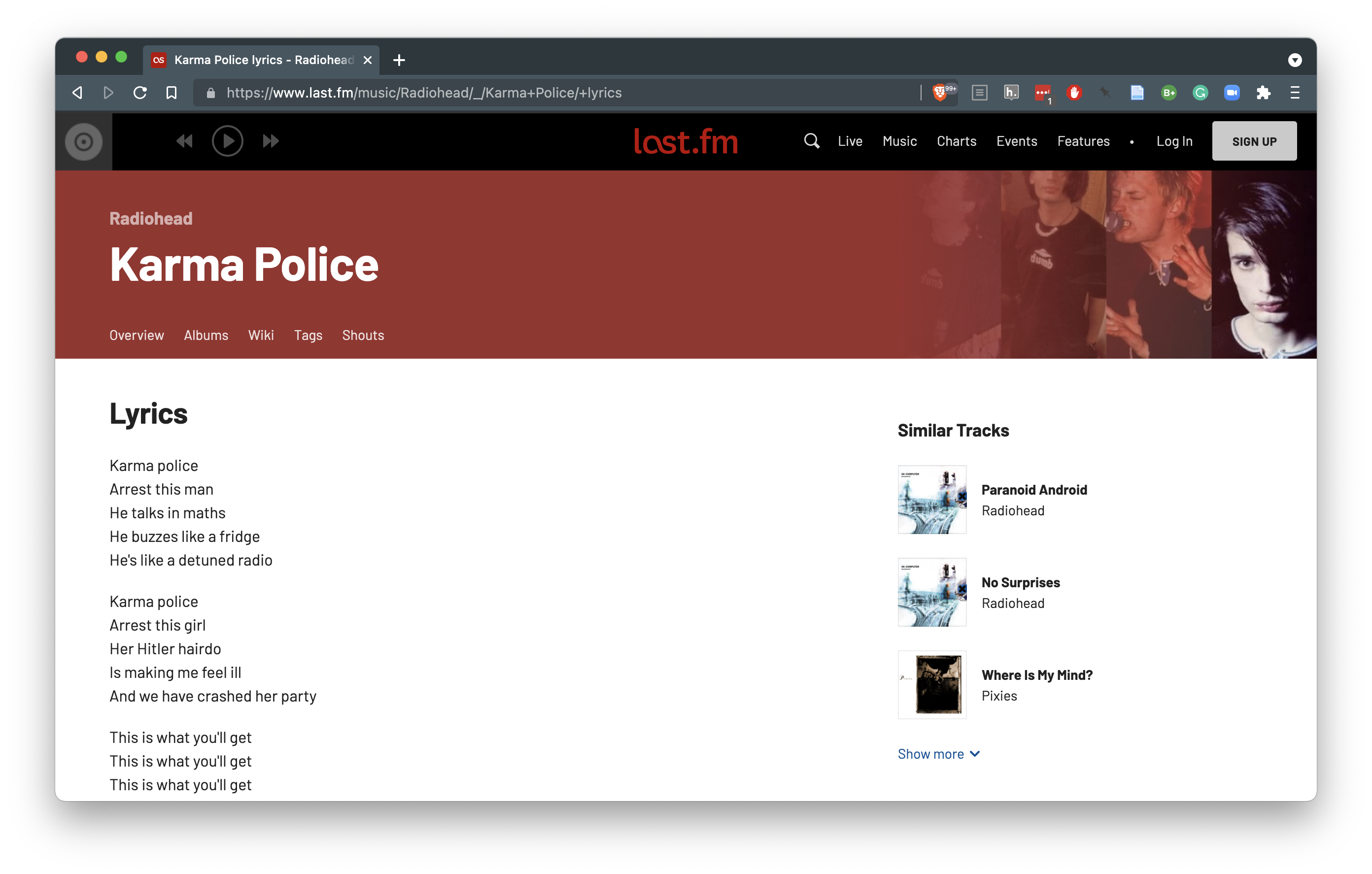
Figure 5.4: Lyrics page from last.fm

As in our toy example, first we want to feed the HTML web address to the read_html() function to parse the tags into elements. We will then assign the result to html.

# read and parse html as an xml object
lyrics_url <- "https://www.last.fm/music/Radiohead/_/Karma+Police/+lyrics"
html <- read_html(lyrics_url)  # read raw html and parse to xml
html

#> {html_document}
#> <html lang="en" class="
#>         no-js
#>         playbar-masthead-release-shim
#>         youtube-provider-not-ready
#>     ">
#> [1] <head>\n<meta http-equiv="Content-Type" content="text/html; charset=UTF-8 ...
#> [2] <body>\n<div id="initial-tealium-data" data-require="tracking/tealium-uta ...

At this point we have captured and parsed the raw HTML assigning it to the object named html. The next step is to identify the html elements that contain the information we want to extract from the page. To do this it is helpful to use a browser to inspect specific elements of the webpage. Your browser will be equipped with a command that you can enable by hovering your mouse over the element of the page you want to target and using a right click to select “Inspect” (Chrome) or “Inspect Element” (Safari, Brave). This will split your browser window vertical or horizontally showing you the raw HTML underlying the webpage.

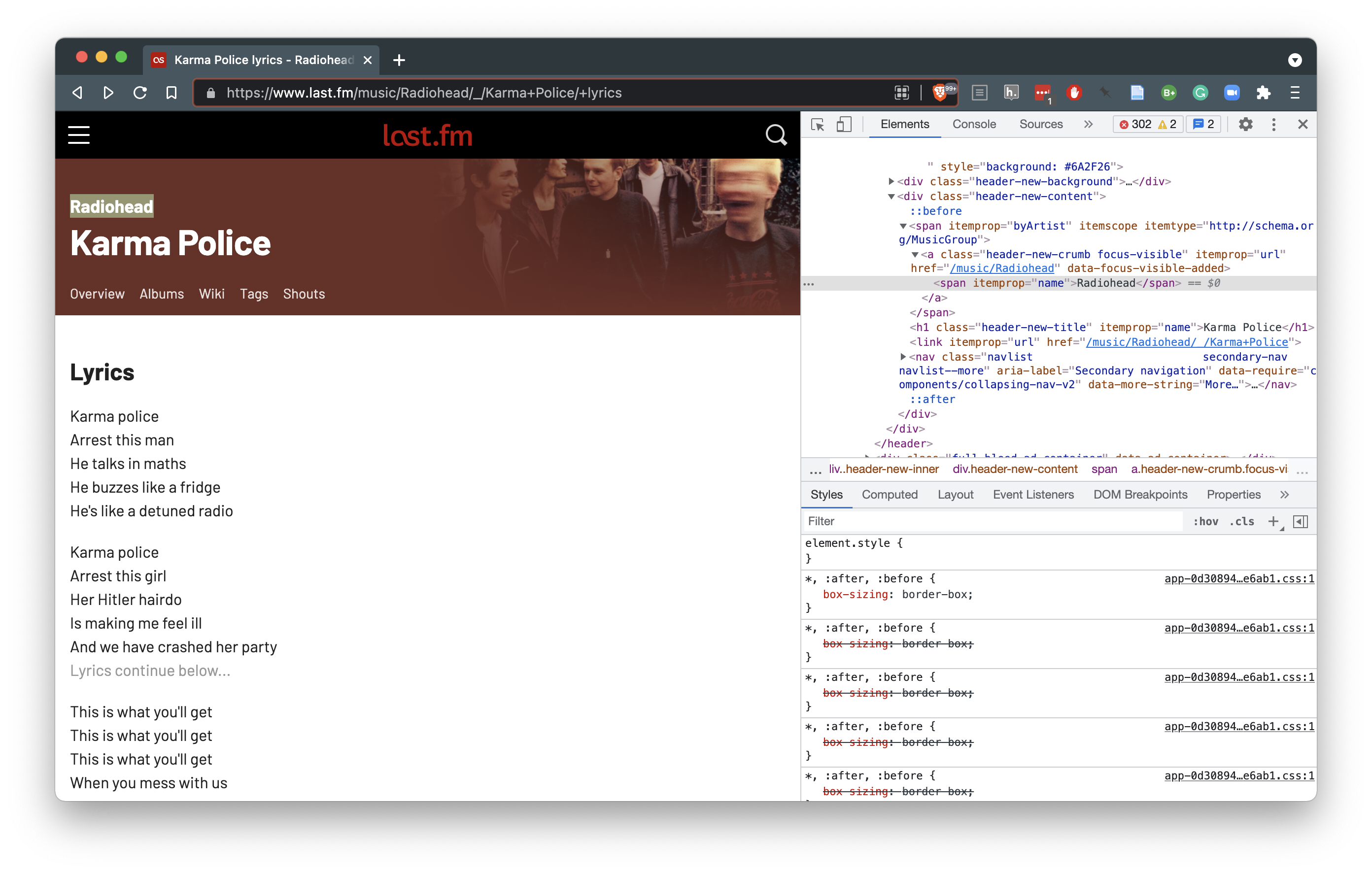
Figure 5.5: Using the “Inspect Element” command to explore raw html.

From Figure 5.6 we see that the element we want to target is contained within an <a></a> tag. Now this tag is common and we don’t want to extract every a so we use the class header-new-crumb to specify we only want the artist name. Using the convention described in our toy example, we can isolate the artist of the lyrics page.

html %>%
    html_element("a.header-new-crumb")
#> {html_node}
#> <a class="header-new-crumb" itemprop="url" href="/music/Radiohead">
#> [1] <span itemprop="name">Radiohead</span>

We can then extract the text with html_text().

artist <- html %>%
    html_element("a.header-new-crumb") %>%
    html_text()
artist
#> [1] "Radiohead"

Let’s extract the song title in the same way.

song <- html %>%
    html_element("h1.header-new-title") %>%
    html_text()
song
#> [1] "Karma Police"

Now if we inspect the HTML of the lyrics page, we will notice that the lyrics are contained in <p></p> tags with the class lyrics-paragraph.

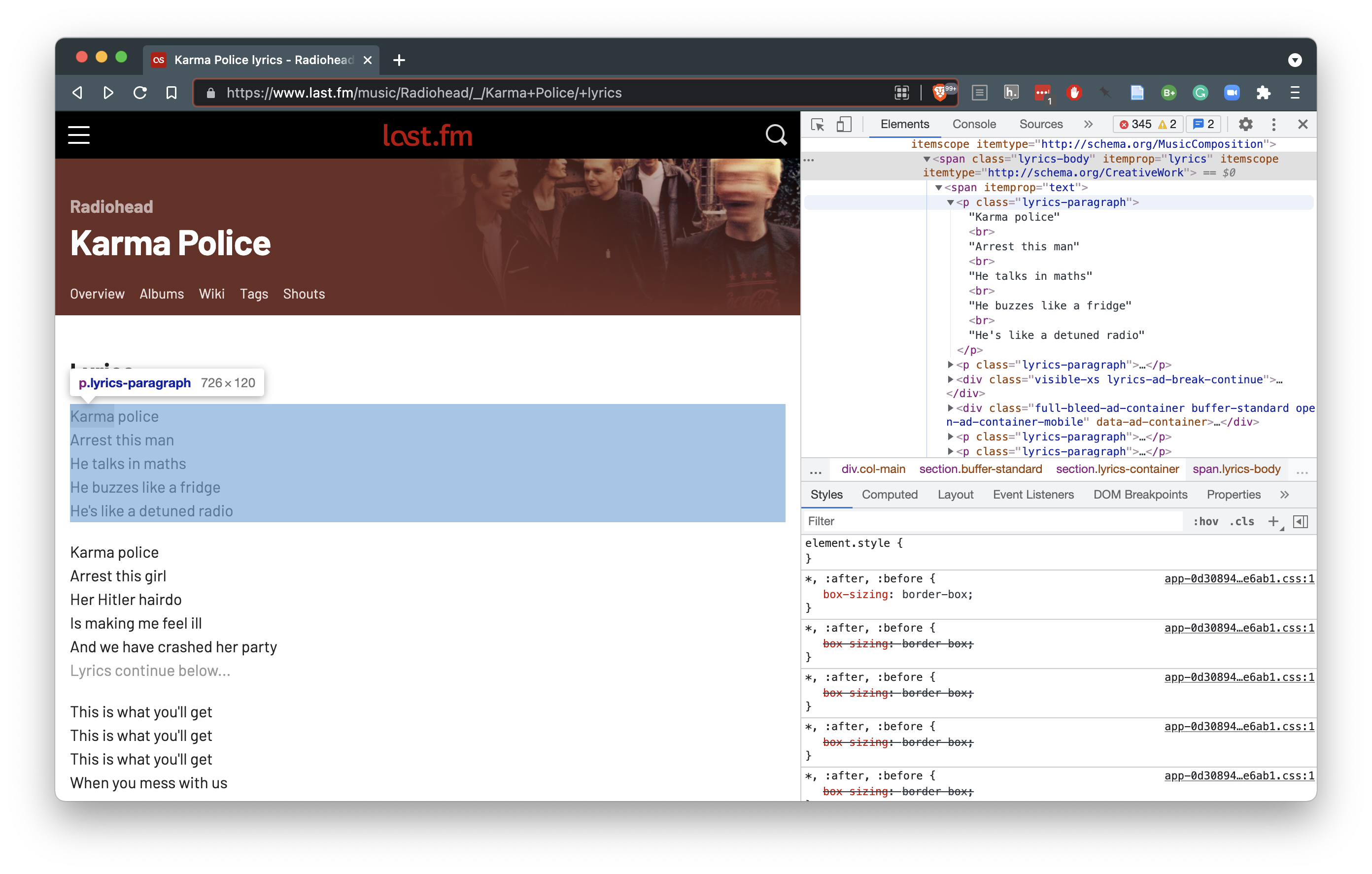
Figure 5.6: Using the “Inspect Element” command to explore raw html.

Since there are multiple elements that we want to extract, we will need to use the html_elements() function instead of the html_element() which only targets one element.

lyrics <- html %>%
    html_elements("p.lyrics-paragraph") %>%
    html_text()
lyrics
#> [1] "Karma policeArrest this manHe talks in mathsHe buzzes like a fridgeHe's like a detuned radio"      
#> [2] "Karma policeArrest this girlHer Hitler hairdoIs making me feel illAnd we have crashed her party"   
#> [3] "This is what you'll getThis is what you'll getThis is what you'll getWhen you mess with us"        
#> [4] "Karma policeI've given all I canIt's not enoughI've given all I canBut we're still on the payroll" 
#> [5] "This is what you'll getThis is what you'll getThis is what you'll getWhen you mess with us"        
#> [6] "For a minute thereI lost myself, I lost myselfPhew, for a minute thereI lost myself, I lost myself"
#> [7] "For a minute thereI lost myself, I lost myselfPhew, for a minute thereI lost myself, I lost myself"

At this point, we have isolated and extracted the artist, song, and lyrics from the webpage. Each of these elements are stored in character vectors in our R session. To complete our task we need to write this data to disk as plain text. With an eye towards a tidy dataset, an ideal format to store the data is in a CSV file where each column corresponds to one of the elements from our scrape and each row an observation. A CSV file is a tabular format and so before we can write the data to disk let’s coerce the data that we have into tabular format. We will use the tibble() function here to streamline our data frame creation. ¹⁹ Feeding each of the vectors artist, song, and lyrics as arguments to tibble() creates the tabular format we are looking for.

tibble(artist, song, lyrics) %>%
    glimpse()
#> Rows: 7
#> Columns: 3
#> $ artist <chr> "Radiohead", "Radiohead", "Radiohead", "Radiohead", "Radiohead"…
#> $ song   <chr> "Karma Police", "Karma Police", "Karma Police", "Karma Police",…
#> $ lyrics <chr> "Karma policeArrest this manHe talks in mathsHe buzzes like a f…

Notice that there are seven rows in this data frame, one corresponding to each paragraph in lyrics. R has a bias towards working with vectors of the same length. As such each of the other vectors (artist, and song) are replicated, or recycled, until they are the same length as the longest vector lyrics, which a length of seven.

For good documentation let’s add our object lyrics_url to the data frame, which contains the actual web link to this page, and assign the result to song_lyrics.

song_lyrics <- tibble(artist, song, lyrics, lyrics_url)

The final step is to write this data to disk. To do this we will use the write_csv() function.

write_csv(x = song_lyrics, path = "../data/original/lyrics.csv")

5.3.3 Scaling up

At this point you may be think, ‘Great, I can download data from a single page, but what about downloading multiple pages?’ Good question. That’s really where the strength of a programming approach takes hold. Extracting information from multiple pages is not fundamentally different than working with a single page. However, it does require more sophisticated understanding of the web and R coding strategies, in particular iteration.

Before we get to iteration, let’s first create a couple functions to make it possible to efficiently reuse the code we have developed so far:

the get_lyrics function wraps the code for scraping a single lyrics webpage from last.fm.

get_lyrics <- function(lyrics_url) {
    # Function: Scrape last.fm lyrics page for: artist, song, and lyrics from a
    # provided content link.  Return as a tibble/data.frame

    cat("Scraping song lyrics from:", lyrics_url, "\n")

    pacman::p_load(tidyverse, rvest)  # install/ load package(s)

    url <- url(lyrics_url, "rb")  # open url connection 
    html <- read_html(url)  # read and parse html as an xml object
    close(url)  # close url connection

    artist <- html %>%
        html_element("a.header-new-crumb") %>%
        html_text()

    song <- html %>%
        html_element("h1.header-new-title") %>%
        html_text()

    lyrics <- html %>%
        html_elements("p.lyrics-paragraph") %>%
        html_text()

    cat("...one moment ")

    Sys.sleep(1)  # sleep for 1 second to reduce server load

    song_lyrics <- tibble(artist, song, lyrics, lyrics_url)

    cat("... done! \n")

    return(song_lyrics)
}

The get_lyrics function includes all of the code developed previously, but also includes: (1) output messages (cat()), (2) a processing pause (Sys.sleep()), and (3) code to manage opening and closing web connections (url() and close()).

Points (1) and (2) will be useful when we iterate over this function to provide status messages and to reduce server load when processing multiple webpages from a web domain. (3) will be necessary to manage webpages that are non-existent. As we will see, we will generate url link to multiple song lyrics some of which will not be valid. To avoid errors that will stop the processing these steps have been incorporated here.

the write_content writes the webscraped data to our local machine, including functionality to create the necessary directory structure of the target file path we choose.

write_content <- function(content, target_file) {
    # Function: Write the tibble content to disk. Create the directory if it
    # does not already exist.

    pacman::p_load(tidyverse)  # install/ load packages

    target_dir <- dirname(target_file)  # identify target file directory structure
    dir.create(path = target_dir, recursive = TRUE, showWarnings = FALSE)  # create directory
    write_csv(content, target_file)  # write csv file to target location

    cat("Content written to disk!\n")
}

With just these two functions, we can take a lyrics URL from last.fm and scrape and write the data to disk like this.

lyrics_url <- "https://www.last.fm/music/Pixies/_/Where+Is+My+Mind%3F/+lyrics"

lyrics_url %>%
    get_lyrics() %>%
    write_content(target_file = "../data/original/lastfm/lyrics.csv")

data/original/lastfm/
└── lyrics.csv

Now we could manually search and copy URLs and run this function pipeline. This would be fine if we had just a few particular URLs that we wanted to scrape. But if we want to, say, scrape a set of lyrics grouped by genre. We would probably want a more programmatic approach. The good news is we can leverage our understanding of webscraping to scrape last.fm to harvest the information needed to create and store links to songs by genre. We can then pass these links to a pipeline, similar to the previous one, to scrape lyrics for many songs and store the results in files grouped by genre.

Last.fm provides a genres page where some of the top genres are listed and can be further explored.

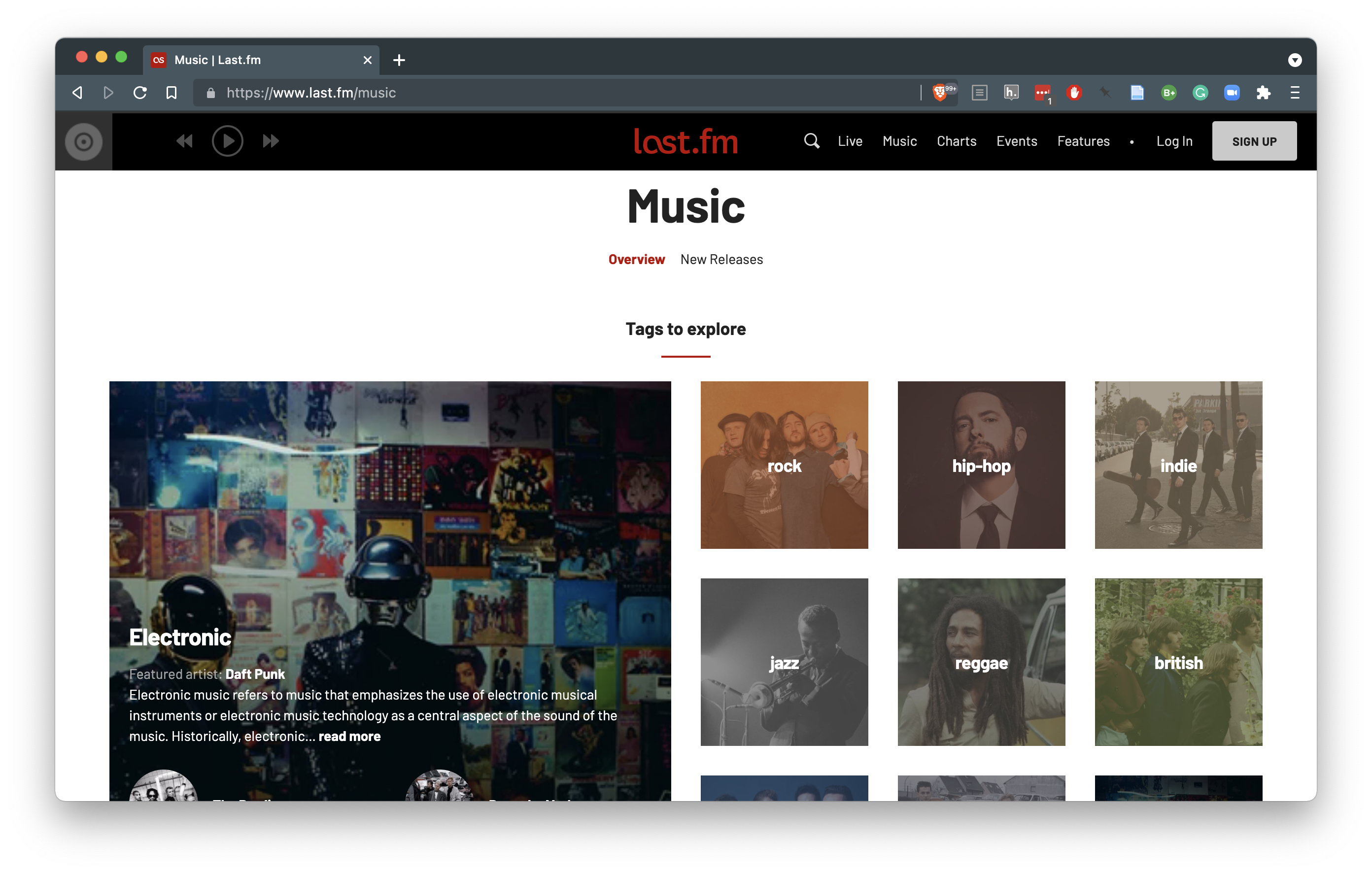
Figure 5.7: Genre page on last.fm

Diving into a a particular genre, ‘rock’ for example, you will get a listing of the top tracks in that genre.

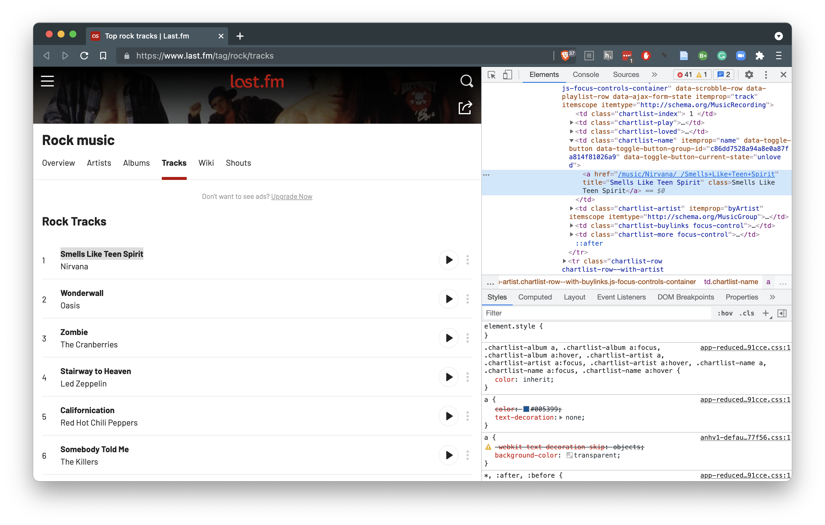
Figure 5.8: Tracks by genre list page on last.fm

If we inspect the HTML elements for the track names in Figure 5.8, we can see that a relative URL is found for the track. In this case, I have ‘Smells Like Teen Spirit’ by Nirvana highlighted in the inspector. If we follow this link to the track page and then to the lyrics for the track, you will notice that the relative URL on the track listings page has all the unique information. Only the web domain https://www.last.fm and the post-pended /+lyrics is missing.

So with this we can put together a function which gets the track listing for a last.fm genre, scrapes the relative URLs for each of the tracks, and creates a full absolute URL to the lyrics page.

get_genre_lyrics_urls <- function(last_fm_genre) {
  # Function: Scrapes a given last.fm genre title for top tracks in
  # that genre and then creates links to the lyrics pages for these tracks
  
  cat("Scraping top songs from:", last_fm_genre, "genre: \n")
  
  pacman::p_load(tidyverse, rvest) # install/ load packages
  
  # create web url for the genre listing page
  genre_listing_url <- 
    paste0("https://www.last.fm/tag/", last_fm_genre, "/tracks") 
  
  genre_lyrics_urls <- 
    read_html(genre_listing_url) %>% # read raw html and parse to xml
    html_elements("td.chartlist-name a") %>% # isolate the track elements
    html_attr("href") %>% # extract the href attribute
    paste0("https://www.last.fm", ., "/+lyrics") # join the domain, relative artist path, and the post-pended /+lyrics to create an absolute URL
  
  return(genre_lyrics_urls)
}

With this function, all we need is to identify the verbatim way last.fm lists the genres. For Rock, it is rock but for Hip Hop, it is hip+hop.

get_genre_lyrics_urls("hip+hop") %>%  # get urls for top hip hop tracks
  head(n = 10) # only display 10 tracks

#> Scraping top songs from: hip+hop genre:
#>  [1] "https://www.last.fm/music/Juzhin/_/Charlie+Conscience+(feat.+MMAIO)/+lyrics"
#>  [2] "https://www.last.fm/music/Juzhin/_/Railways/+lyrics"                        
#>  [3] "https://www.last.fm/music/Juzhin/_/Coming+Down/+lyrics"                     
#>  [4] "https://www.last.fm/music/Juzhin/_/Tupona/+lyrics"                          
#>  [5] "https://www.last.fm/music/Juzhin/_/Sakhalin/+lyrics"                        
#>  [6] "https://www.last.fm/music/Juzhin/_/3+Simple+Minutes/+lyrics"                
#>  [7] "https://www.last.fm/music/Juzhin/_/Lost+Sense/+lyrics"                      
#>  [8] "https://www.last.fm/music/Juzhin/_/Wonderful/+lyrics"                       
#>  [9] "https://www.last.fm/music/Gina+Moryson/_/Vanilla+Smoothy+(Live)/+lyrics"    
#> [10] "https://www.last.fm/music/Juzhin/_/Flunk-Down+(Juzhin+Remix)/+lyrics"

So now we have a method to scrape URLs by genre and list them in a vector. Our approach, then, could be to pass these lyrics URLs to our existing pipeline which downloads the lyrics (get_lyrics()) and then writes them to disk (write_content()).

# Note: will not run
get_genre_lyrics_urls("hip+hop") %>% # get lyrics urls for specific genre
  get_lyrics() %>% # scrape lyrics url
  write_content(target_file = "../data/original/lastfm/hip_hop.csv") # write to disk

This approach, however, has a couple problems. (1) our get_lyrics() function only takes one URL at a time, but the result of get_genre_lyrics_urls() will produce many URLs. We will be able to solve this with iteration using the purrr package, specifically the map() function which will iteratively map each URL output from get_genre_lyrics_urls() to get_lyrics() in turn. (2) the output from our iterative application of get_lyrics() will produce a tibble for each URL, which then sets up a problem with writing the tibbles to disk with the write_content() function. To avoid this we will want to combine the tibbles into one single tibble and then send it to be written to disk. The bind_rows() function will do just this.

# Note: will run, but with occasional errors
get_genre_lyrics_urls("hip+hop") %>% # get lyrics urls for specific genre
  map(get_lyrics) %>%  # scrape lyrics url
  bind_rows() %>% # combine tibbles into one
  write_content(target_file = "../data/original/lastfm/hip_hop.csv") # write to disk

This preceding pipeline conceptually will work. However, on my testing, it turns out that some of the URLs that are generated in the get_genre_lyrics_urls() do not exist on the site. That is, the song is listed but no lyrics have been added to the song site. This will mean that when the URL is sent to the get_lyrics() function, there will be an error when attempting to download and parse the page with read_html() which will halt the entire process. To avoid this error, we can wrap the get_lyrics() function in a function designed to attempt to download and parse the URL (tryCatch()), but if there is an error, it will skip it and move on to the next URL without stopping the processing. This approach is reflected in the get_lyrics_catch() function below.

# Wrap the `get_lyrics()` function with `tryCatch()` to skip URLs that have no
# lyrics

get_lyrics_catch <- function(lyrics_url) {
    tryCatch(get_lyrics(lyrics_url), error = function(e) return(NULL))  # no, URL, return(NULL)/ skip
}

Updating the pipeline with the get_lyrics_catch() function would look like this:

# Note: will run, but we can do better
get_genre_lyrics_urls("hip+hop") %>% # get lyrics urls for specific genre
  map(get_lyrics_catch) %>%  # scrape lyrics url
  bind_rows() %>% # combine tibbles into one
  write_content(target_file = "../data/original/lastfm/hip_hop.csv") # write to disk

This will work, but as we have discussed before one of this goals we have we acquiring data for a reproducible research project is to make sure that we are developing efficient code that will not burden site’s server we are scraping from. In this case, we would like to check to see if the data is already downloaded. If not, then the script should run. If so, then the script does not run. Of course this is a perfect use of a conditional statement. To make this a single function we can call, I’ve wrapped the functions we created for getting lyric URLs from last.fm, scraping the URLs, and writing the results to disk in the download_lastfm_lyrics() function below. I also added a line to add a last_fm_genre column to the combined tibble to store the name of the genre we scraped (i.e. mutate(genre = last_fm_genre).

download_lastfm_lyrics <- function(last_fm_genre, target_file) {
    # Function: get last.fm lyric urls by genre and write them to disk

    if (!file.exists(target_file)) {

        cat("Downloading data.\n")

        get_genre_lyrics_urls(last_fm_genre) %>%
            map(get_lyrics_catch) %>%
            bind_rows() %>%
            mutate(genre = last_fm_genre) %>%
            write_content(target_file)

    } else {
        cat("Data already downloaded!\n")
    }
}

Now we can call this function on any genre on the last.fm site and download the top 50 song lyrics for that genre (provided they all have lyrics pages).

# Scrape lyrics for 'pop'
download_lastfm_lyrics(last_fm_genre = "pop", target_file = "../data/original/lastfm/pop.csv")

# Scrape lyrics for 'rock'
download_lastfm_lyrics(last_fm_genre = "rock", target_file = "../data/original/lastfm/rock.csv")

# Scrape lyrics for 'hip hop'
download_lastfm_lyrics(last_fm_genre = "hip+hop", target_file = "../data/original/lastfm/hip_hop.csv")

# Scrape lyrics for 'metal'
download_lastfm_lyrics(last_fm_genre = "metal", target_file = "../data/original/lastfm/metal.csv")

Now we can see that our web scrape data is organized in a similar fashion to the other data we acquired in this chapter.

data/
├── derived/
└── original/
    ├── cedel2/
    │   └── texts.csv
    ├── gutenberg/
    │   ├── works_pq.csv
    │   └── works_pr.csv
    ├── lastfm/
    │   ├── country.csv
    │   ├── hip_hop.csv
    │   ├── lyrics.csv
    │   ├── metal.csv
    │   ├── pop.csv
    │   └── rock.csv
    ├── sbc/
    │   ├── meta-data/
    │   └── transcriptions/
    ├── scs/
    │   ├── README
    │   ├── discourse
    │   ├── disfluency
    │   ├── documentation/
    │   ├── tagged
    │   ├── timed-transcript
    │   └── transcript
    └── twitter/
        └── rt_latinx.csv

Again, it is important to add these custom functions to our acquire_functions.R script in the functions/ directory so we can access them in our scripts more efficiently and make our analysis steps more succinct and legible.

In this section we covered scraping language data from the web. The rvest package provides a host of functions for downloading and parsing HTML. We first looked at a toy example to get a basic understanding of how HTML works and then moved to applying this knowledge to a practical example. To maintain a reproducible workflow, the code developed in this example was grouped into task-oriented functions which were in turn joined and wrapped into a function that provided convenient access to our workflow and avoided unnecessary downloads (in the case the data already exists on disk).

Here we have built on previously introduced R coding concepts and demonstrated various others. Web scraping often requires more knowledge of and familiarity with R as well as other web technologies. Rest assured, however, practice will increase confidence in your abilities. I encourage you to practice on your own with other websites. You will encounter problems. Consult the R documentation in RStudio or online and lean on the R community on the web at sites such as Stack Overflow inter alia.

5.4 Documentation

As part of the data acquisition process it is important include documentation that describes the data resource(s) that will serve as the base for a research project. For all resources the data should include as much information possible that outlines the sampling frame of the data (Ädel, 2020). For a corpus sample acquired from a repository will often include documentation which will outline the sampling frame –this most likely will be the very information which leads a researcher to select this resource for the project at hand. It is important to include this documentation (HTML or PDF file) or reference to the documentation (article citation or link²⁰) within the reproducible project’s directory structure.

In other cases where the data acquisition process is formulated and conducted by the researcher for the specific aims of the research (i.e. API and web scraping approaches), the researcher should make an effort to document those aspects which are key for the study, but that may also be of interest to other researchers for similar research questions. This will may include language characteristics such as modality, register, genre, etc., speaker/ writer characteristics such as demographics, time period(s), context of the linguistic communication, etc. and process characteristics such as the source of the data, the process of acquisition, date of acquisition, etc. However, it is important to recognize that each language sample and the resource from which it is drawn is unique. As a general rule of thumb, a researcher should document the resource as if this were a resource they were to encounter for the first time. To archive this information, it is standard practice to include a README file in the relevant directory where the data is stored.

data/
├── derived/
└── original/
    ├── cedel2/
    │   ├── documentation/
    │   └── texts.csv
    ├── gutenberg/
    │   ├── README.md
    │   ├── works_pq.csv
    │   └── works_pr.csv
    ├── lastfm/
    │   ├── README.md
    │   ├── country.csv
    │   ├── hip_hop.csv
    │   ├── lyrics.csv
    │   ├── metal.csv
    │   ├── pop.csv
    │   └── rock.csv
    ├── sbc/
    │   ├── meta-data/
    │   └── transcriptions/
    ├── scs/
    │   ├── README
    │   ├── discourse
    │   ├── disfluency
    │   ├── documentation/
    │   ├── tagged
    │   ├── timed-transcript
    │   └── transcript
    └── twitter/
        ├── README.md
        └── rt_latinx.csv

For both existing corpora and data samples acquired by the researcher it is also important to signal if there are conditions and/ or licensing restrictions that one should heed when using and potentially sharing the data. In some cases existing corpus data come with restrictions on data sharing. These can be quite restrictive and ultimately require that the corpus data not be included in publically available reproducible project or data can only be shared in a derived format. If this the case, it is important to document the steps to legally acquire the data so that a researcher can acquire their own license and take full advantage of your reproducible project.

In the case of data from APIs or web scraping, there too may be stipulations on sharing data. A growing number of data sources apply one of the available Creative Common Licenses. Check the source of your data for more information and if you are a member of a research institution you will likely have a specialist on Copyright and Fair Use.

Summary

In this chapter we have covered a lot of ground. On the surface we have discussed three methods for acquiring corpus data for use in text analysis. In the process we have delved into various aspects of the R programming language. Some key concepts include writing custom functions and working with those function in an iterative manner. We have also considered topics that are more general in nature and concern interacting with data found on the internet.

Each of these methods should be approached in a way that is transparent to the researcher and to would-be collaborators and the general research community. For this reason the documentation of the steps taken to acquire data are key both in the code and in human-facing documentation.

At this point you have both a bird’s eye view of the data available on the web and strategies on how to access a great majority of it. It is now time to turn to the next step in our data analysis project: data curation. In the next posts I will cover how to wrangle your raw data into a tidy dataset. This will include working with and incorporating meta-data as well as augmenting a dataset with linguistic annotations.

Overview

6 Curate data(sets)