10 Exploration
INCOMPLETE DRAFT
Nobody ever figures out what life is all about, and it doesn’t matter. Explore the world. Nearly everything is really interesting if you go into it deeply enough.
– Richard P. Feynman
The essential questions for this chapter are:
- …
In this chapter….
identify, interrogate, and interpret
EDA is an inductive approach. That is, it is bottom-up –we do not come into the analysis with strong preconceptions of what the data will tell us (IDA - hypothesis and PDA - target classes). The aim is to uncover and discover patterns that lead to insight based on qualitative interpretation. EDA, the, can be considered a quantitative-supported qualitative analysis.
-
Two main classes of exploratory data analysis: (1) descriptive analysis and (2) unsupervised machine learning.
- descriptive analysis can be seen as a more detailed implementation of descriptive assessment, which is a key component of both inferential and predictive analysis approaches. .
- unsupervised machine learning is a more algorithmic approach to deriving knowledge which leverages … to produce knowledge which can be interpreted. This approach falls under the umbrella of machine learning, as we have seen in predictive data analysis, however, whereas PDA assumes a potential relationship between input features and target outcomes, or classes, in unsupervised learning the classes are induced from the data itself and the classes groupings are interpreted and evaluated more …?
It is, however, important to come to EDA with a research question in which the unit of analysis is clear.
Description of the datasets we will use to examine various exploratory methods.
Lastfm
Last.fm webscrape of the top artists by genre which we acquired in Chapter 5 “Acquire data” in the web scrape section and transformed in Chapter 6 “Transform data”.
glimpse(lastfm_df)  # preview dataset structure
#> Rows: 200
#> Columns: 4
#> $ artist <chr> "Alan Jackson", "Alan Jackson", "Brad Paisley", "Carrie Underwo…
#> $ song   <chr> "Little Bitty", "Remember When", "Mud on the Tires", "Before He…
#> $ lyrics <chr> "Have a little love on a little honeymoon You got a little dish…
#> $ genre  <chr> "country", "country", "country", "country", "country", "country…
The lastfm_df dataset contains 155 observations and 4 variables. Each observation corresponds to a particular song.
Let’s look at the data dictionary for this dataset.
| variable_name | name | description |
|---|---|---|
| artist | Artist Name | The name of the artist |
| song | Song Title | The title of the song |
| lyrics | Song Lyrics | The lyrics for the song |
| genre | Song Genre | The genre of the artist (source last.fm) |
From the data dictionary we see that each song encodes the artist, the song title, the genre of the song, and the lyrics for the song.
To prepare for the upcoming exploration methods, we will convert the lastfm_df to a Quanteda corpus object.
# Create corpus object
lastfm_corpus <-
  lastfm_df %>% # data frame
  corpus(text_field = "lyrics") # create corpus

lastfm_corpus %>%
  summary(n = 5) # preview
#> Corpus consisting of 155 documents, showing 5 documents:
#>
#>   Text Types Tokens Sentences           artist                song   genre
#>  text1    84    271         1     Alan Jackson        Little Bitty country
#>  text2   110    203         1     Alan Jackson       Remember When country
#>  text3   130    290         2     Brad Paisley    Mud on the Tires country
#>  text4   114    303         1 Carrie Underwood    Before He Cheats country
#>  text5   171    517        15   Dierks Bentley What Was I Thinkin' country
SOTU
The quanteda package (Benoit et al., 2022) includes various datasets. We will work with the State of the Union Corpus (Benoit, 2020). Let’s take a look at the structure of this dataset.
glimpse(sotu_df)  # preview dataset structure
#> Rows: 84
#> Columns: 5
#> $ president <chr> "Truman", "Truman", "Truman", "Truman", "Truman", "Truman", …
#> $ delivery  <fct> written, spoken, spoken, spoken, spoken, spoken, spoken, wri…
#> $ party     <fct> Democratic, Democratic, Democratic, Democratic, Democratic, …
#> $ year      <dbl> 1946, 1947, 1948, 1949, 1950, 1951, 1952, 1953, 1953, 1954, …
#> $ text      <chr> "To the Congress of the United States:\n\nA quarter century …
In the sotu_df dataset there are 84 observations and 5 variables. Each observation corresponds to a presidential address.
Let’s look at the data dictionary to understand what each column measures.
| variable_name | name | description |
|---|---|---|
| president | President | Incumbent president |
| delivery | Modality of delivery | Modality of the address (spoken or written) |
| party | Political party | Party affliliation of the president |
| year | Year | Year that the statement was given |
| text | Text | Text or transcription of the address |
So we see that each observation corresponds to the president that gave the address, the modality of the address, the party the president was affliated with, the year that the address was given, and the address text.
10.1 Descriptive analysis
… overview summary of the aims of descriptive analysis methods…
10.1.1 Frequency analysis
Explore word frequency.
# Create tokens object
lastfm_tokens <-
  lastfm_corpus %>% # corpus object
  tokens(what = "word", # tokenize by word
         remove_punct = TRUE) %>% # remove punctuation
  tokens_tolower() # lowercase tokens

lastfm_tokens %>%
  head(n = 1) # preview one tokenized document
#> Tokens consisting of 1 document and 3 docvars.
#> text1 :
#>  [1] "have"      "a"         "little"    "love"      "on"        "a"
#>  [7] "little"    "honeymoon" "you"       "got"       "a"         "little"
#> [ ... and 252 more ]
We see the tokenized output.
Many of the frequency analysis function provided with quanteda require that the dataset be in a document-frequency matrix. So let’s create a dfm of the lastfm_corpus object using the dfm() function.
# Create document-frequency matrix
lastfm_dfm <-
  lastfm_tokens %>% # tokens object
  dfm() # create dfm

lastfm_dfm %>%
  head(n = 5) # preview 5 documents
#> Document-feature matrix of: 5 documents, 3,966 features (97.19% sparse) and 3 docvars.
#>        features
#> docs    have  a little love on honeymoon you got dish and
#>   text1    1 35     34    1  5         1   4   3    1  10
#>   text2    0  1      1    3  0         0   3   0    0  12
#>   text3    1 21     11    0  9         0   6   5    0   6
#>   text4    1 10      5    0  3         0   1   0    0   4
#>   text5    0 22      7    0  2         0   0   1    0   5
#> [ reached max_nfeat ... 3,956 more features ]
Frequency distributions.
- Very few high frequency terms and many low frequency.
- This results in a long tail when plotted.
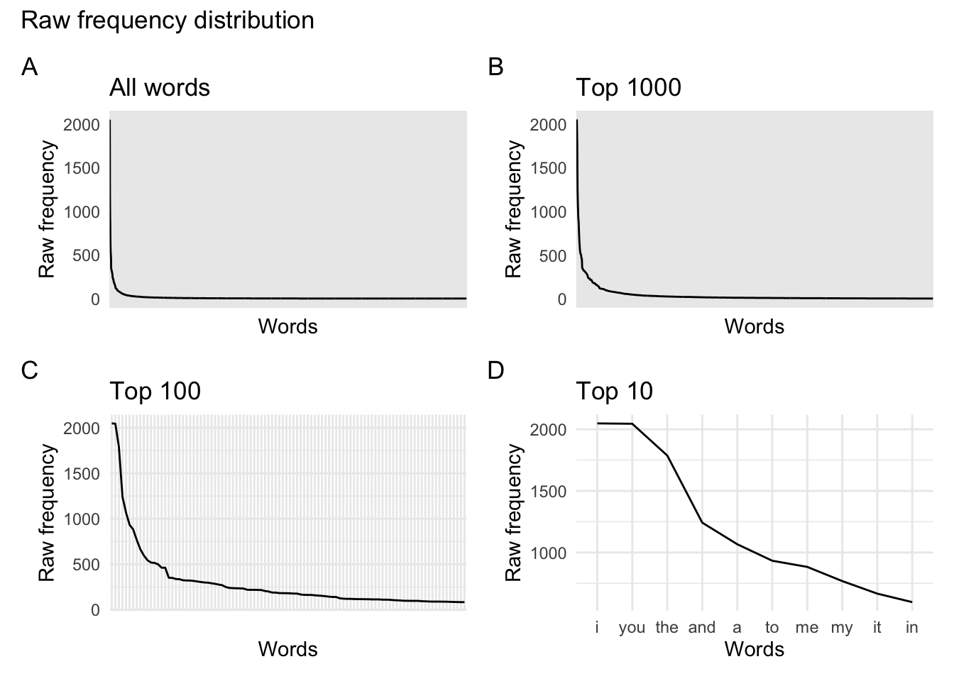
Let’s take a closer look at the 50 most frequent word terms in lastfm_dfm. We use the textstat_frequency() function from the quanteda.textstats package to extract various frequency measures.
lastfm_dfm %>%
    textstat_frequency() %>%
    slice_head(n = 10)
#>    feature frequency rank docfreq group
#> 1        i      2048    1     148   all
#> 2      you      2045    2     139   all
#> 3      the      1787    3     148   all
#> 4      and      1242    4     151   all
#> 5        a      1067    5     135   all
#> 6       to       933    6     147   all
#> 7       me       883    7     132   all
#> 8       my       768    8     116   all
#> 9       it       666    9     118   all
#> 10      in       597   10     131   all
We can then use this data frame to plot the frequency of the terms in descending order using ggplot().
lastfm_dfm %>%
textstat_frequency() %>%
slice_head(n = 50) %>%
ggplot(aes(x = reorder(feature, frequency), y = frequency)) + geom_col() + coord_flip() +
labs(x = "Words", y = "Raw frequency", title = "Top 50")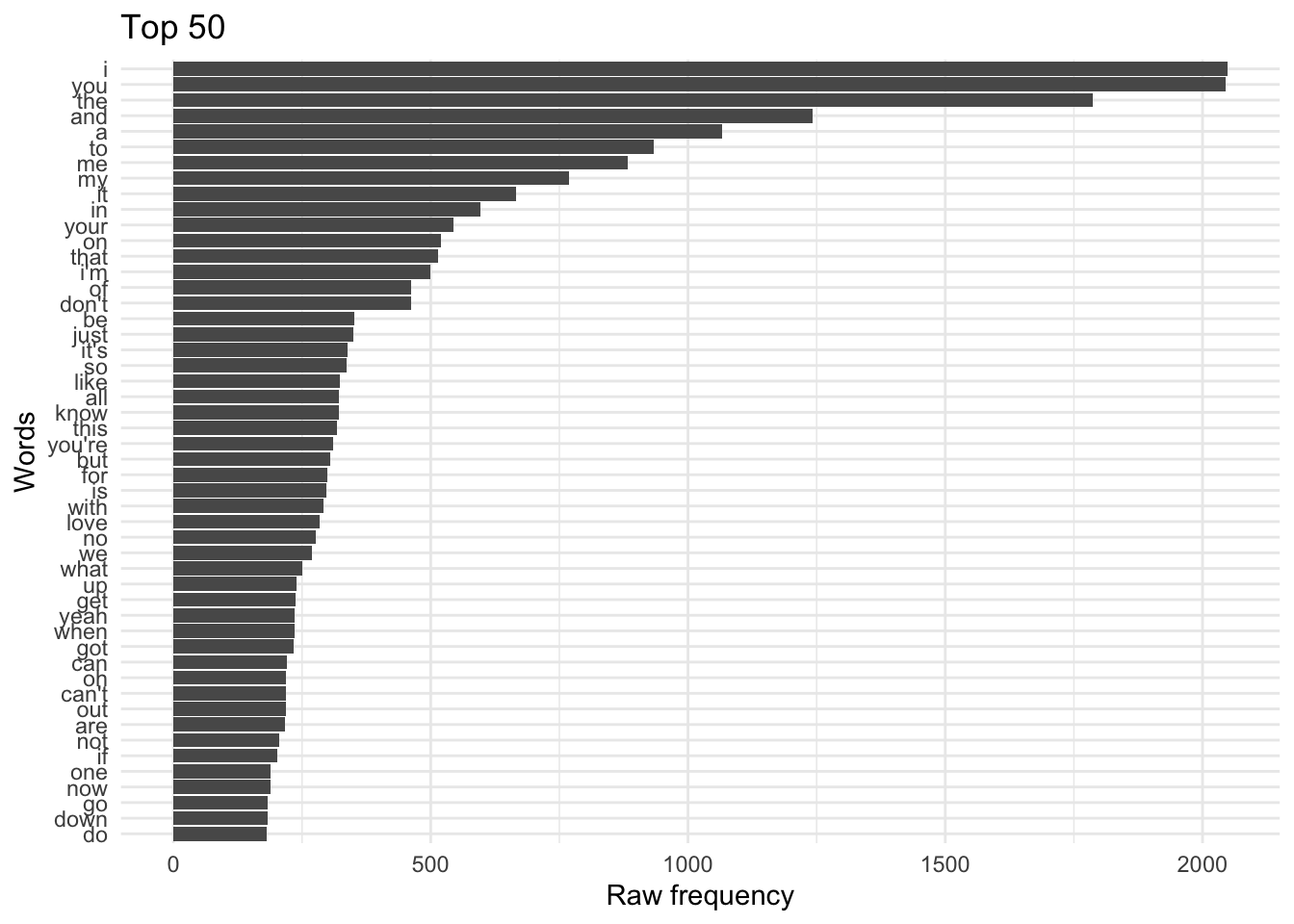 Now these are the most common terms for all of the song lyrics. In our case, let’s look at the most common 15 terms for each of the genres. We will need at a
 groups = argument to textstat_frequency() to get the genre and then we need to manipulate the data frame output and the extract the top 15 terms grouping by genre.
lastfm_dfm %>% # dfm
  textstat_frequency(groups = genre) %>% # get frequency statistics
  group_by(group) %>% # grouping parameters
  slice_max(frequency, n = 15) %>% # extract top features
  ungroup() %>% # remove grouping parameters
  ggplot(aes(x = frequency, y = reorder_within(feature, frequency, group), fill = group)) + # mappings (reordering feature by frequency)
  geom_col(show.legend = FALSE) + # bar plot
  scale_y_reordered() + # clean up y-axis labels (features)
  facet_wrap(~group, scales = "free_y") + # organize separate plots by genre
  labs(x = "Raw frequency", y = NULL) # labels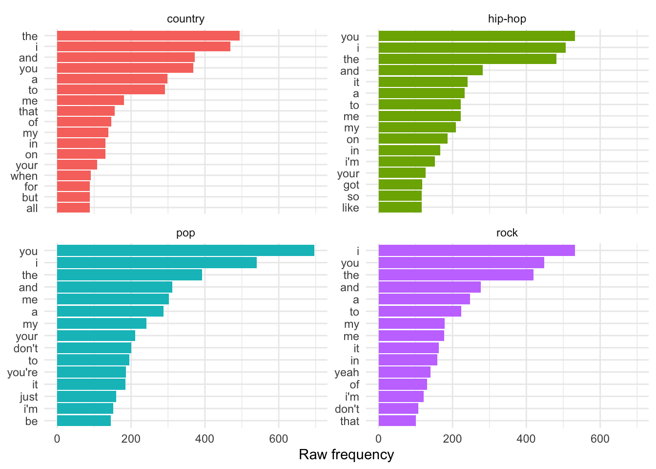
Note that I’ve used the plotting function facet_wrap() to tell ggplot2 to organize each of the genres in separate bar plots but in the same plotting space. The scales = argument takes either free, free_x, or free_y as a value. This will let the all the axes or either the x- or y-axis vary freely between the separate plots.
Raw frequency is effected by the total number of words in each genre. Therefore we cannot safely make direct comparisons between the frequency counts for individual terms between genres.
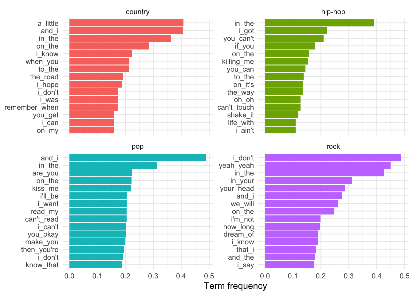
To make the term-genre comparisons comparable we normalized the term frequency by the number of terms in each genre. We can use the dfm_weight() function with the argument scheme = "prop" to give us the relative frequency of a term per the number of terms in the document it appears in. This weighting is known as Term frequency.
lastfm_dfm %>% # dfm
  dfm_weight(scheme = "prop") %>% # weigh by term frequency
  textstat_frequency(groups = genre) %>% # get frequency statistics
  group_by(group) %>% # grouping parameters
  slice_max(frequency, n = 15) %>% # extract top features
  ungroup() %>% # remove grouping parameters
  ggplot(aes(x = frequency, y = reorder_within(feature, frequency, group), fill = group)) + # mappings (reordering feature by frequency)
  geom_col(show.legend = FALSE) + # bar plot
  scale_y_reordered() + # clean up y-axis labels (features)
  facet_wrap(~group, scales = "free_y") + # organize separate plots by genre
  labs(x = "Term frequency", y = NULL) # labels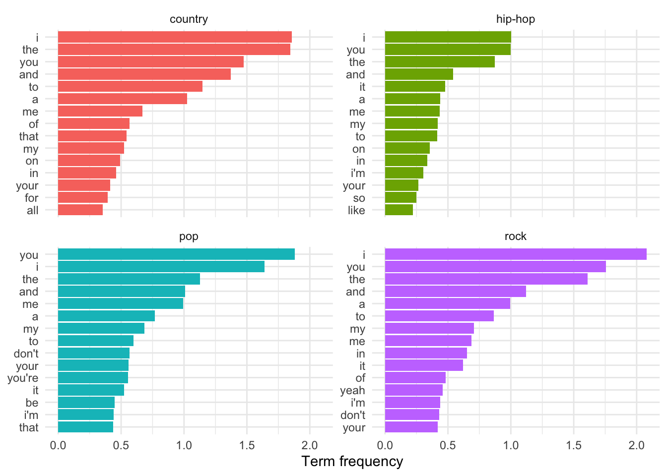
Term frequency makes the frequency scores relative to the genre. This means that the frequencies are directly comparable as the number of words in each genre is taken into account when calculating the term frequency score.
Now our term frequency measures allow us to make direct comparisons, but one problem here is that the most frequent terms tend to be terms that are common across all language use. Since the aim of most frequency analyses which compare sub-groups is to discover what terms are most indicative of each sub-group we need a way to adjust or weigh our measures. The scheme often applied to scale terms according to how common they are is to apply term frequency-inverse document frequency (tf-idf). The tf-idf measure is the result of multiplying the term frequency by the inverse document frequency.
lastfm_df %>% # data frame
  count(genre) %>%  # get number of documents for each genre
  select(Genre = genre, `Number of documents` = n) %>%
  knitr::kable(booktabs = TRUE,
caption = "Number of documents per genre.")| Genre | Number of documents |
|---|---|
| country | 44 |
| hip-hop | 26 |
| pop | 41 |
| rock | 44 |
lastfm_dfm %>%
  dfm_weight(scheme = "prop") %>% # term-frequency weight
  textstat_frequency(groups = genre) %>% # include genre as a group
  filter(feature == "i") # filter only "i"
#>      feature frequency rank docfreq   group
#> 1          i      1.86    1      42 country
#> 1639       i      1.00    1      26 hip-hop
#> 3600       i      1.64    2      38     pop
#> 5012       i      2.08    1      42    rock
# Manually calculate TF-IDF scores
1.86 * log10(44/42)  # i in country
#> [1] 0.0376
1 * log10(26/26)  # i in hip hop
#> [1] 0
1.64 * log10(41/38)  # i in pop
#> [1] 0.0541
2.08 * log10(44/42)  # i in rock
#> [1] 0.042
lastfm_dfm %>%
    dfm_tfidf(scheme_tf = "prop") %>%
    textstat_frequency(groups = genre, force = TRUE) %>%
    filter(str_detect(feature, "^(i|yeah)$")) %>%
    arrange(feature)
#>      feature frequency rank docfreq   group
#> 213        i    0.0373  213      42 country
#> 1873       i    0.0201  235      26 hip-hop
#> 3842       i    0.0329  244      38     pop
#> 5197       i    0.0417  186      42    rock
#> 239     yeah    0.0350  239       8 country
#> 1742    yeah    0.0336  104      14 hip-hop
#> 3755    yeah    0.0454  157      13     pop
#> 5013    yeah    0.2165    2      17    rock
lastfm_dfm %>% # dfm
  dfm_tfidf(scheme_tf = "prop") %>%  # weigh by tf-idf
  textstat_frequency(groups = genre, force = TRUE) %>% # get frequency statistics
  group_by(group) %>% # grouping parameters
  slice_max(frequency, n = 15) %>% # extract top features
  ungroup() %>% # remove grouping parameters
  ggplot(aes(x = frequency, y = reorder_within(feature, frequency, group), fill = group)) + # mappings (reordering feature by frequency)
  geom_col(show.legend = FALSE) + # bar plot
  scale_y_reordered() + # clean up y-axis labels (features)
  facet_wrap(~group, scales = "free_y") + # organize separate plots by genre
  labs(x = "TF-IDF", y = NULL) # labels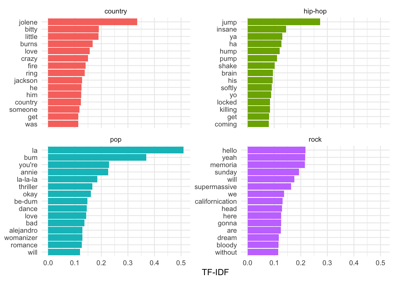
TF-IDF works well to identify terms which are particularly indicative of a particular group but there is a shortcoming which is particularly salient when working with song lyrics. That is, that there are terms which are frequent but not common because they appear in one song and are repeated. This is common in song lyrics which tend to have repeated chorus sections. To minimize this influence, we can trim the document-frequency matrix and eliminate terms which only appear in one song.
lastfm_dfm %>% # dfm
dfm_trim(min_docfreq = 2) %>% # keep terms appearing in 2 or more songs
dfm_tfidf(scheme_tf = "prop") %>% # weigh by tf-idf
textstat_frequency(groups = genre, force = TRUE) %>% # get frequency statistics
group_by(group) %>% # grouping parameters
slice_max(frequency, n = 15) %>% # extract top features
ungroup() %>% # remove grouping parameters
ggplot(aes(x = frequency, y = reorder_within(feature, frequency, group), fill = group)) + # mappings (reordering feature by frequency)
geom_col(show.legend = FALSE) + # bar plot
scale_y_reordered() + # clean up y-axis labels (features)
facet_wrap(~group, scales = "free_y") + # organize separate plots by genre
labs(x = "TF-IDF", y = NULL) # labels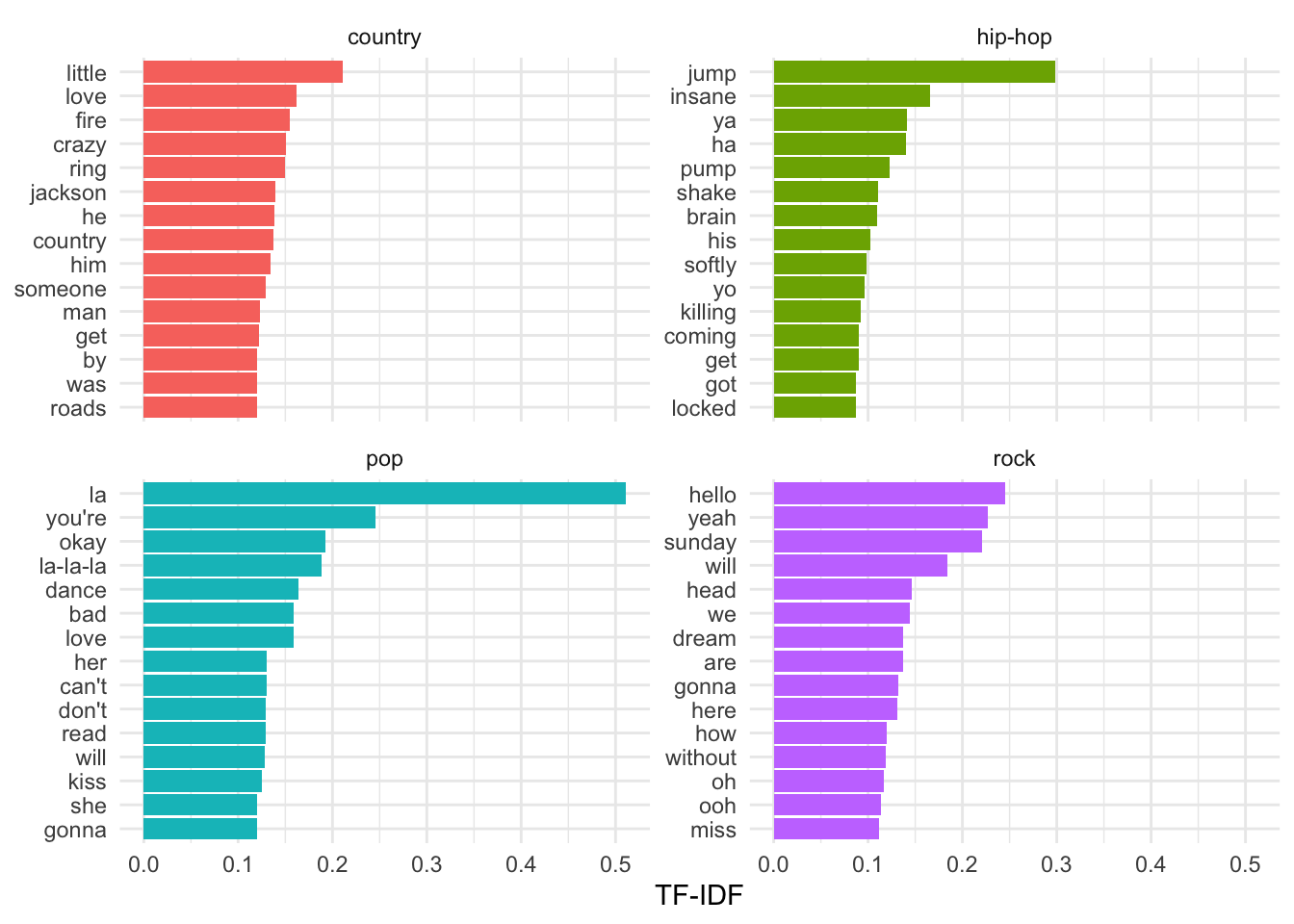 Now we are looking a terms which are indicative of their respective genres and appear in at least 2 songs.
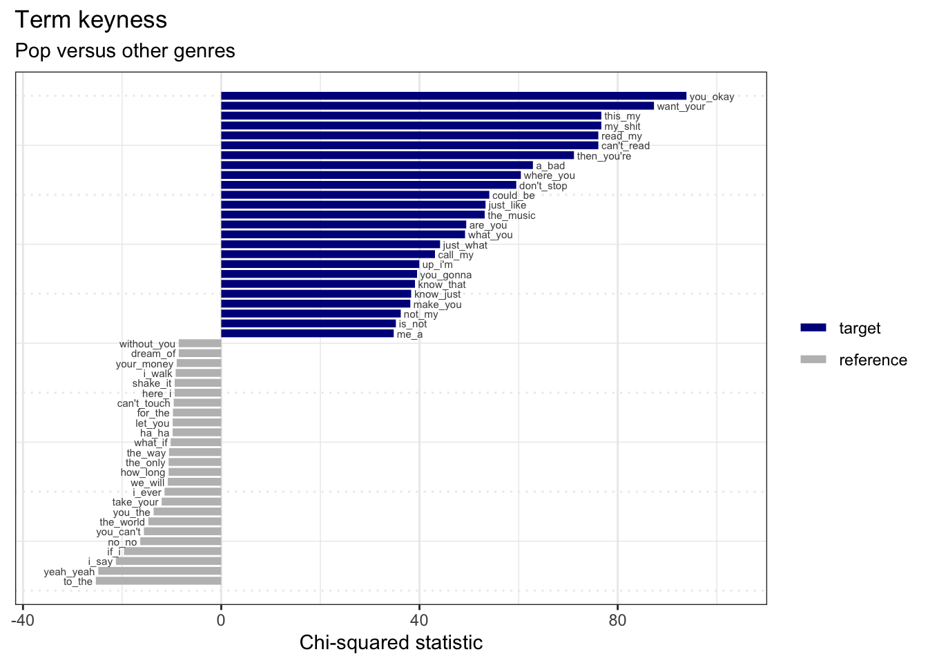
Another exploration method is to look at relative frequency, or keyness, measures. This type of analysis compares the relative frequency of terms of a target group in comparison to a reference group. If we set the target to one of our genres then the other genres become the reference. The results show which terms occur significantly more often than they occur in the reference group(s). The textstat_keyness() function implements this type of analysis in quanteda.
lastfm_keywords_country <-
  lastfm_dfm %>% # dfm
  dfm_trim(min_docfreq = 2) %>% # keep terms appearing in 2 or more songs
  textstat_keyness(target = lastfm_dfm$genre == "country") # compare country

lastfm_keywords_country %>%
  slice_head(n = 10) # preview
#>    feature  chi2        p n_target n_reference
#> 1   little 113.3 0.00e+00       77          43
#> 2   belong  45.6 1.46e-11       19           4
#> 3     ring  45.2 1.80e-11       22           7
#> 4     he's  43.3 4.82e-11       25          11
#> 5     went  43.2 4.90e-11       17           2
#> 6     fire  42.2 8.24e-11       21           7
#> 7    blues  42.2 8.44e-11       14           0
#> 8      him  40.9 1.60e-10       34          24
#> 9  country  38.8 4.58e-10       13           0
#> 10    road  37.7 8.11e-10       23          11
The output of the textstat_keyness() function all terms from most frequent in the target group to the most frequent in the reference group(s). The textplot_keyness() takes advantage of this and we can see the most contrastive terms in a plot.
Let’s look at what terms are most and least indicative of the ‘country’ genre.
lastfm_keywords_country %>%
  textplot_keyness(n = 25, labelsize = 2) + # plot most contrastive terms
  labs(x = "Chi-squared statistic",
       title = "Term keyness",
       subtitle = "Country versus other genres") # labels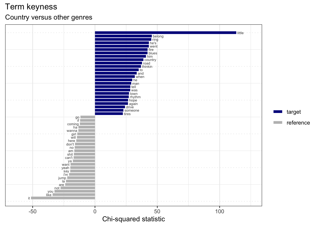
Interpretation….
Now let’s look at the ‘Hip hop’ genre.
lastfm_dfm %>% # dfm
  dfm_trim(min_docfreq = 2) %>% # keep terms appearing in 2 or more songs
  textstat_keyness(target = lastfm_dfm$genre == "hip-hop") %>% # compare hip hop
  textplot_keyness(n = 25, labelsize = 2) + # plot most contrastive terms
  labs(x = "Chi-squared statistic",
      title = "Term keyness",
       subtitle = "Hip hop versus other genres") # labels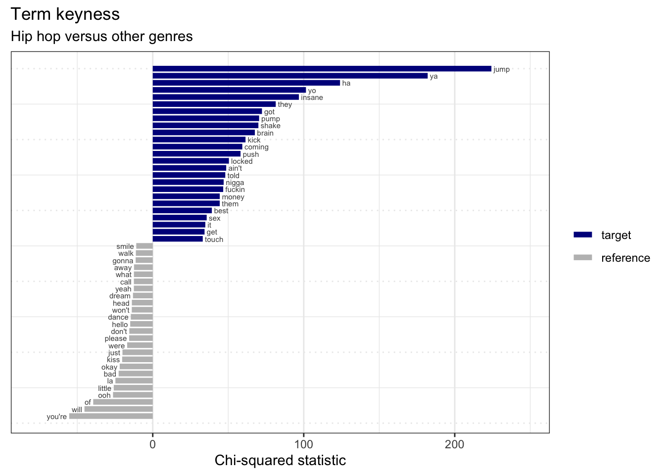
Interpretation …
Now we have been working with words as our tokens/ features but a word is simply a unigram token. We can also consider multi-word tokens, or ngrams. To create bigrams (2-word tokens) we return to the lastfm_tokens object and add the function tokens_ngrams() with the argument n = 2 (for bigrams). Then just as before we create a DFM object. I will go ahead and trim the DFM to exclude terms appearing only in one document (i.e. song).
# Tokenize by bigrams
lastfm_dfm_ngrams <-
  lastfm_tokens %>% # word tokens
  tokens_ngrams(n = 2) %>% # create 2-term ngrams (bigrams)
  dfm() %>% # create document-frequency matrix
  dfm_trim(min_docfreq = 2) # keep terms appearing in 2 or more songs

lastfm_dfm_ngrams %>%
  head(n = 1) # preview 1 document
#> Document-feature matrix of: 1 document, 3,232 features (98.73% sparse) and 3 docvars.
#>        features
#> docs    have_a a_little on_a you_got got_a and_you and_a well_it's it's_alright
#>   text1      1       25    1       3     3       1     7         2            4
#>        features
#> docs    to_be
#>   text1     4
#> [ reached max_nfeat ... 3,222 more features ]
Interpretation …
We can now repeat the same steps we did earlier to explore raw frequency, term frequency, and tf-idf frequency measures by genre. We will skip the visualization of raw frequency as it is inherently incompatible with direct comparisons between sub-groups.
Interpretation …
We can even pull out particular terms and explore them directly.
# Term frequency comparison
lastfm_dfm_ngrams %>%
    dfm_weight(scheme = "prop") %>%
    textstat_frequency(groups = genre) %>%
    filter(str_detect(feature, "i_ain't"))
#>      feature frequency rank docfreq   group
#> 45   i_ain't     0.110   45       4 country
#> 1944 i_ain't     0.109   15       8 hip-hop
#> 3733 i_ain't     0.109   54       3     pop
Interpretation …

Before we leave this introduction to frequency analysis, let’s consider another type of metric which can be used to explore term usage in and across documents which aims to estimate lexical diversity, the number of unique terms (types) to the total number of terms (tokens). This is known as the Type-Token Ratio (TTR). The TTR measure is biased when comparison documents or groups differ in the number of total tokens. To mitigate this issue the Moving-Average Type-Token Ratio (MATTR) is often used. MATTR the moving window size must be set to a reasonable size given the size of the documents. In this case we will use 50 as all the lyrics in the datasset have at least this number of words.
I will use box plots to visualize the distribution of the TTR and MATTR estimates across the four genres.
lastfm_lexdiv <- lastfm_tokens %>%
    textstat_lexdiv(measure = c("TTR", "MATTR"), MATTR_window = 50)

lastfm_docvars <- lastfm_tokens %>%
    docvars()

lastfm_lexdiv_meta <- cbind(lastfm_docvars, lastfm_lexdiv)

p1 <- lastfm_lexdiv_meta %>%
    ggplot(aes(x = reorder(genre, TTR), y = TTR, color = genre)) + geom_boxplot(notch = TRUE,
    show.legend = FALSE) + labs(x = "Genre")

p2 <- lastfm_lexdiv_meta %>%
    ggplot(aes(x = reorder(genre, MATTR), y = MATTR, color = genre)) + geom_boxplot(notch = TRUE,
    show.legend = FALSE) + labs(x = "Genre")

p1 + p2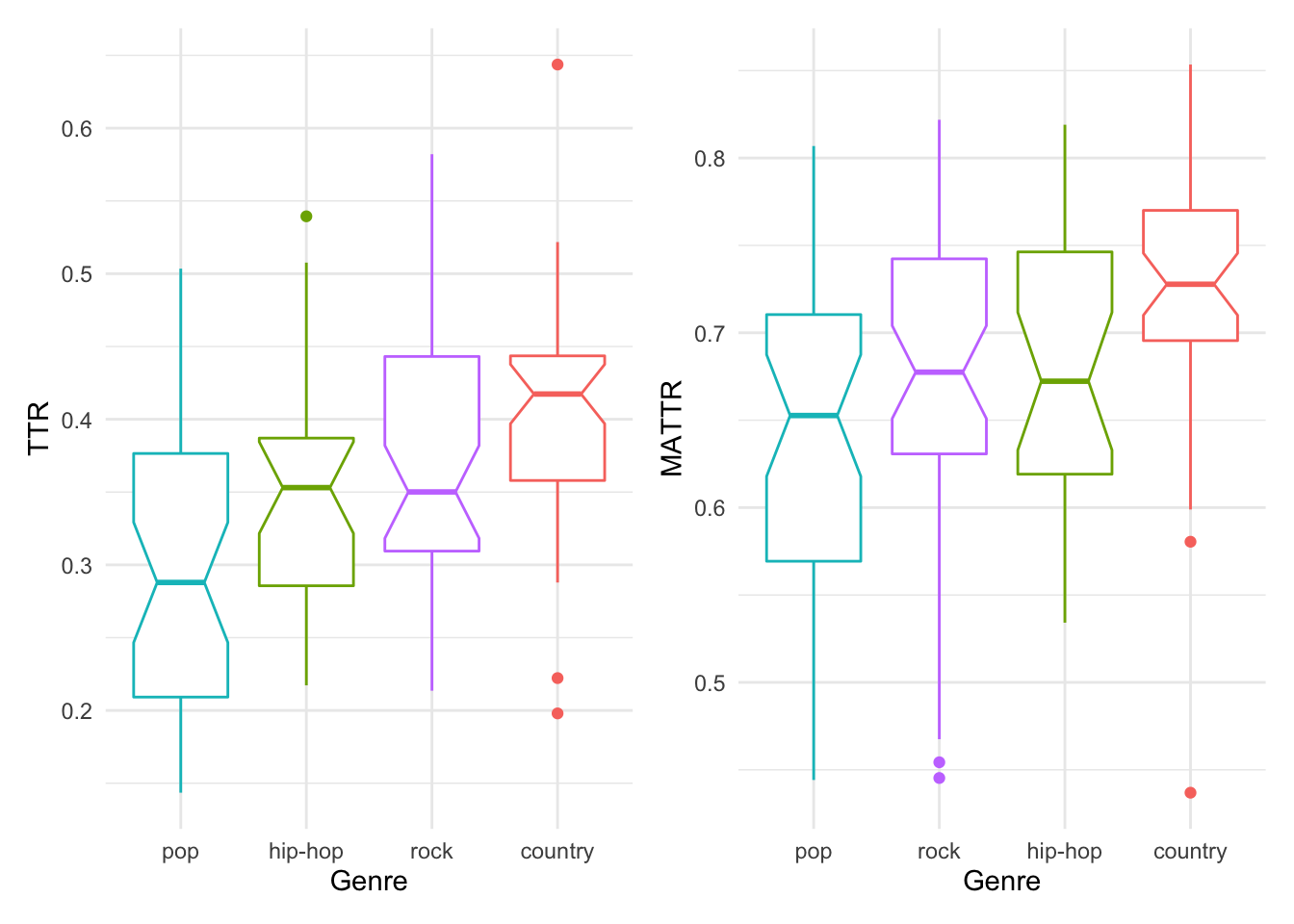
We can see that there are similarities and differences between the two estimates of lexical diversity. In both cases, there is a trend towards ‘country’ being the most diverse and ‘pop’ the least diverse. ‘rock’ and ‘hip-hop’ are swapped given the estimate type. It is important, however, to note that the notches in the box plot provide us a rough guide to gauge whether these trends are statistically significant or not. Focusing on the more reliable MATTR and using the notches as our guide, it looks like we can safely say that ‘country’ is more lexically diverse than the other genres. Another potential take-home message is that pop appears to be the most internally variable –that is, there appears to be quite a bit of variability between the lexical diversity in songs in this genre.
10.1.2 Collocation analysis
Where frequency analysis focuses on the usage of terms, collocation analysis focuses on the usage of terms in context.
- Keyword in Context
kwic()
lastfm_tokens %>%
    tokens_group(groups = genre) %>%
    kwic(pattern = "ain't") %>%
    slice_sample(n = 10)
#> Keyword-in-context with 10 matches.
#>   [country, 4468]       to find another for it | ain't |
#>   [hip-hop, 6158]         i got lyrics but you | ain't |
#>     [hip-hop, 66]         i'm into havin sex i | ain't |
#>       [pop, 3060]     happen like that cause i | ain't |
#>    [hip-hop, 336]         i'm into havin sex i | ain't |
#>   [country, 9027]            no pool no pets i | ain't |
#>   [hip-hop, 9996]     in his cage the audience | ain't |
#>  [hip-hop, 10005]     ain't gone clap and they | ain't |
#>    [hip-hop, 378]         i'm into havin sex i | ain't |
#>   [hip-hop, 5398] maybe we're crazy probably i | ain't |
#>
#>  right that she should live
#>  got none if you come
#>  into makin love so come
#>  no hollaback girl i ain't
#>  into makin love so come
#>  got no cigarettes ah but
#>  fazed and they ain't gone
#>  gone praise they want everything
#>  into makin love so come
#>  happy i'm feeling glad i
You can also search for multiword expressions using phrase(). You can use a pattern matching convention to make your key term searches more (‘glob’ and ‘regex’) or less (‘fixed’) flexible.
lastfm_tokens %>%
    tokens_group(groups = genre) %>%
    kwic(pattern = phrase("ain't no*"), valuetype = "glob") %>%
    slice_sample(n = 10)
#> Keyword-in-context with 10 matches.
#>    [hip-hop, 171:172]        they wanna fuck but homie | ain't nothing |
#>  [hip-hop, 3345:3346]        streets it's the d-r-e it | ain't nothing |
#>      [pop, 3451:3452]         happen like that cause i |   ain't no    |
#>      [pop, 3065:3066]        ain't no hollaback girl i |   ain't no    |
#>    [pop, 10320:10321] is thriller thriller night there |   ain't no    |
#>      [pop, 3231:3232]        ain't no hollaback girl i |   ain't no    |
#>      [pop, 3060:3061]         happen like that cause i |   ain't no    |
#>  [country, 2758:2759]            i'm a redneck woman i |   ain't no    |
#>      [pop, 3368:3369]         happen like that cause i |   ain't no    |
#>      [pop, 3373:3374]        ain't no hollaback girl i |   ain't no    |
#>
#>  change hoes down g's up
#>  but more hot shit another
#>  hollaback girl i ain't no
#>  hollaback girl a few times
#>  second chance against the thing
#>  hollaback girl ooh ooh this
#>  hollaback girl i ain't no
#>  high class broad i'm just
#>  hollaback girl i ain't no
#> hollaback girl ooh ooh this- Collocation analysis
The frequency analysis of ngrams as terms is similar to but distinct from a collocation analysis. In a collocation analysis the frequency with which a two or more terms co-occur is balanced by the frequency of the terms when they do not cooccur. In other words, the sequences occur more than one would expect given the frequency of the individual terms. This provides an estimate of the tendency of a sequence of words to form a cohesive semantic or syntactic unit.
We can apply the textstat_collocations() function on a tokens object (lastfm_tokens) and retrieve the most cohesive collocations (using the \(z\)-statistic) for the entire dataset.
lastfm_tokens %>%
    textstat_collocations() %>%
    slice_head(n = 5)
#>   collocation count count_nested length lambda    z
#> 1      in the   227            0      2   2.95 33.4
#> 2   yeah yeah    86            0      2   5.32 33.4
#> 3   jump jump    64            0      2   8.44 28.0
#> 4       oh oh    59            0      2   4.78 27.8
#> 5     bum bum    44            0      2   7.48 26.7
Add a minimum frequency count (min_count =) to avoid hapaxes (terms which happen infrequently yet when they do occur, the cooccur with another specific term which also occurs infrequently). We can also specify the size of the collocation (the default is 2). If we set it to 3 then we will get three-word collocations.
lastfm_tokens %>%
    textstat_collocations(min_count = 50, size = 2) %>%
    slice_head(n = 10)
#>    collocation count count_nested length lambda    z
#> 1       in the   227            0      2   2.95 33.4
#> 2    yeah yeah    86            0      2   5.32 33.4
#> 3    jump jump    64            0      2   8.44 28.0
#> 4        oh oh    59            0      2   4.78 27.8
#> 5        la la    59            0      2   9.13 25.5
#> 6      i'm not    64            0      2   3.95 25.0
#> 7     a little    76            0      2   4.45 23.3
#> 8      i don't   140            0      2   2.40 23.1
#> 9       on the   131            0      2   2.29 22.0
#> 10      like a    81            0      2   2.82 21.4
If we want to explore the collocations for a specific group in our dataset, we can use the tokens_subset() function and specify the group that we want to subset and use. Note that the minimum count will need to be lowered (if used at all) as the size of the dataset is now a fraction of what is was when we considered all the documents (not just those from a particular genre).
lastfm_tokens %>%
    tokens_subset(genre == "pop") %>%
    textstat_collocations(min_count = 10, size = 3) %>%
    slice_head(n = 25)
#>        collocation count count_nested length lambda    z
#> 1         of you i    12            0      3   6.85 6.35
#> 2     i just can't    16            0      3   5.98 4.80
#> 3         cry me a    27            0      3   8.81 4.03
#> 4        up on you    10            0      3   4.01 4.00
#> 5        is not my    17            0      3   7.11 3.84
#> 6    you know that    19            0      3   2.71 3.77
#> 7   don't stop the    25            0      3   7.01 3.76
#> 8   know just just    14            0      3   7.55 3.61
#> 9       you and me    11            0      3   5.16 3.44
#> 10  just just what    14            0      3   7.14 3.43
#> 11  don't you like    13            0      3   5.16 3.42
#> 12    are you okay    40            0      3   6.98 3.37
#> 13     just like a    27            0      3   5.58 3.35
#> 14 where you gonna    27            0      3   5.90 3.30
#> 15    i'm not your    10            0      3   6.80 3.28
#> 16        my no he    10            0      3   7.85 3.16
#> 17        me and i    10            0      3   2.45 3.15
#> 18   don't call my    18            0      3   6.36 3.09
#> 19   gonna be okay    10            0      3   7.59 3.06
#> 20    this my shit    33            0      3   7.46 3.00
#> 21  dance gonna be    10            0      3   7.28 2.94
#> 22  because of you    14            0      3   6.19 2.90
#> 23   just what you    14            0      3   2.94 2.90
#> 24   for your call    11            0      3   5.97 2.84
#> 25      am the one    12            0      3   6.05 2.84
In this section we have covered some common strategies for doing exploration with descriptive analysis methods. These methods can be extended and combined to dig into and uncover patterns as the research and intermediate findings dictate.
10.2 Unsupervised learning
We now turn our attention to a second group of methods for conducting exploratory analyses –unsupervised learning.
- Clustering
textstat_dist()
library(factoextra)

lastfm_clust <- lastfm_dfm %>%
    dfm_weight(scheme = "prop") %>%
    textstat_dist(method = "euclidean") %>%
    as.dist() %>%
    hclust(method = "ward.D2")

lastfm_clust %>%
    fviz_dend(show_labels = FALSE, k = 4)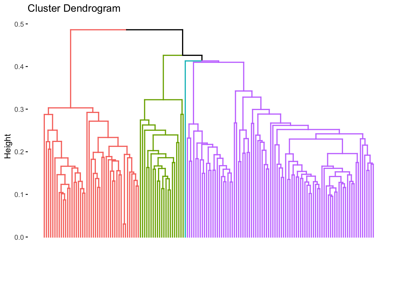

clusters <- lastfm_clust %>%
    cutree(k = 3) %>%
    as_tibble(rownames = "document")

clusters
#> # A tibble: 155 × 2
#>    document value
#>    <chr>    <int>
#>  1 text1        1
#>  2 text2        2
#>  3 text3        2
#>  4 text4        1
#>  5 text5        1
#>  6 text6        2
#>  7 text7        3
#>  8 text8        2
#>  9 text9        1
#> 10 text10       1
#> # … with 145 more rows
docvars(lastfm_dfm, field = "cluster") <- clusters$value
lastfm_dfm$cluster <- clusters$value

lastfm_dfm %>%
    docvars %>%
    head
#>             artist                song   genre cluster
#> 1     Alan Jackson        Little Bitty country       1
#> 2     Alan Jackson       Remember When country       2
#> 3     Brad Paisley    Mud on the Tires country       2
#> 4 Carrie Underwood    Before He Cheats country       1
#> 5   Dierks Bentley What Was I Thinkin' country       1
#> 6     Dolly Parton              9 to 5 country       2
lastfm_dfm %>%
    docvars() %>%
    janitor::tabyl(genre, cluster) %>%
    janitor::adorn_totals(where = c("row", "col")) %>%
    janitor::adorn_percentages() %>%
    janitor::adorn_pct_formatting()
#>    genre     1     2     3  Total
#>  country 47.7% 40.9% 11.4% 100.0%
#>  hip-hop 69.2% 19.2% 11.5% 100.0%
#>      pop 63.4% 19.5% 17.1% 100.0%
#>     rock 54.5% 31.8% 13.6% 100.0%
#>    Total 57.4% 29.0% 13.5% 100.0%
Looking at the assigned clusters and the genres of the songs we see some interesting patterns. For one cluster 1 appears to have the majority of the songs, followed by cluster 2, and 3. In cluster 1 Hip hop and Pop make up the majority of the songs. In cluster 2 Country and Rock tend to dominate and in cluster 3 there is a scattering of genres.
Now we can approach this again with distinct linguistic unit. Where in our current clusters we used words, we could switch to bigrams and see if the results change and how they change.
# Clustering: bigram features- Topic modeling
# textmodel_lsa()- Sentiment analysis