9 Prediction
INCOMPLETE DRAFT
…
The essential questions for this chapter are:
- …
- …
- …
In this chapter we will
Orientation to the question(s) and dataset(s) to be explored …
wricle_df <- read_csv(file = "resources/10-prediction/data/derived/wricle_formal_curated.csv")

locness_df <- read_csv(file = "resources/10-prediction/data/derived/locness_curated.csv")
learners_df <- wricle_df %>%
    filter(native_language == "Spanish") %>%
    mutate(student = "Spanish") %>%
    mutate(type = "Learner") %>%
    select(essay_id = id, type, student, essay)

glimpse(learners_df)
#> Rows: 689
#> Columns: 4
#> $ essay_id <chr> "A1-1", "A1-2", "A10-1", "A10-2", "A101-1", "A101-2", "A101-3…
#> $ type     <chr> "Learner", "Learner", "Learner", "Learner", "Learner", "Learn…
#> $ student  <chr> "Spanish", "Spanish", "Spanish", "Spanish", "Spanish", "Spani…
#> $ essay    <chr> "In our present society gay people is asking for the same rig…
natives_df <- locness_df %>%
    unite(col = doc_id, c("file_id", "essay_id"), sep = "-") %>%
    mutate(doc_id = str_replace(doc_id, "\\.txt", "")) %>%
    mutate(type = "Native") %>%
    select(essay_id = doc_id, type, student, essay)

glimpse(natives_df)
#> Rows: 411
#> Columns: 4
#> $ essay_id <chr> "alevels1-1", "alevels1-2", "alevels1-3", "alevels1-4", "alev…
#> $ type     <chr> "Native", "Native", "Native", "Native", "Native", "Native", "…
#> $ student  <chr> "British", "British", "British", "British", "British", "Briti…
#> $ essay    <chr> "The basic dilema facing the UK's rail and road transport sys…
nativeness_df <- rbind(learners_df, natives_df) # combine
nativeness_df %>%
    unnest_tokens(output = "word", input = "essay") %>%
    count(word, type) %>%
    group_by(type) %>%
    summarize(total_words = sum(n))
#> # A tibble: 2 × 2
#>   type    total_words
#>   <chr>         <int>
#> 1 Learner      640535
#> 2 Native       324269
nativeness_corpus <- nativeness_df %>%
    corpus(text_field = "essay")

nativeness_corpus_summary <- nativeness_corpus %>%
    summary(n = ndoc(nativeness_corpus))

nativeness_corpus_summary %>%
    slice_head(n = 10)
#> Corpus consisting of 1100 documents, showing 1100 documents:
#>
#>    Text Types Tokens Sentences essay_id    type student
#>   text1   210    496        26     A1-1 Learner Spanish
#>   text2   253    655        29     A1-2 Learner Spanish
#>   text3   280    722        30    A10-1 Learner Spanish
#>   text4   177    389        15    A10-2 Learner Spanish
#>   text5   245    636        19   A101-1 Learner Spanish
#>   text6   219    692        17   A101-2 Learner Spanish
#>   text7   213    615        16   A101-3 Learner Spanish
#>   text8   319    914        23   A101-4 Learner Spanish
#>   text9   253    654        19   A102-1 Learner Spanish
#>  text10   310    816        21   A102-2 Learner Spanish
nativeness_corpus$doc_id <- 1:ndoc(nativeness_corpus)

nativeness_corpus %>%
    docvars() %>%
    slice_head(n = 5)
#>   essay_id    type student doc_id
#> 1     A1-1 Learner Spanish      1
#> 2     A1-2 Learner Spanish      2
#> 3    A10-1 Learner Spanish      3
#> 4    A10-2 Learner Spanish      4
#> 5   A101-1 Learner Spanish      5
nativeness_tokens <- nativeness_corpus %>%
    tokens(what = "word", remove_punct = TRUE, remove_numbers = TRUE, remove_symbols = TRUE)

nativeness_tokens %>%
    tokens_group(groups = type) %>%
    head()
#> Tokens consisting of 2 documents and 1 docvar.
#> Learner :
#>  [1] "In"      "our"     "present" "society" "gay"     "people"  "is"
#>  [8] "asking"  "for"     "the"     "same"    "rights"
#> [ ... and 636,407 more ]
#>
#> Native :
#>  [1] "The"       "basic"     "dilema"    "facing"    "the"       "UK's"
#>  [7] "rail"      "and"       "road"      "transport" "system"    "is"
#> [ ... and 321,936 more ]
nativeness_dfm <- nativeness_tokens %>%
    dfm()

nativeness_dfm %>%
    head(n = 5)
#> Document-feature matrix of: 5 documents, 28,129 features (99.24% sparse) and 4 docvars.
#>        features
#> docs    in our present society gay people is asking for the
#>   text1 12   5       4       5   5     10 12      1   3  23
#>   text2 26   2       1       4   0     10 14      0   1  45
#>   text3 12   4       0       4   9     16 12      0   0  12
#>   text4 15   1       0       1   0      9  7      0   1  10
#>   text5 15   1       1       2   0      7 17      0   6  40
#> [ reached max_nfeat ... 28,119 more features ]

nativeness_dfm %>%
    dfm_group(groups = type) %>%
    head(n = 5)
#> Document-feature matrix of: 2 documents, 28,129 features (33.74% sparse) and 1 docvar.
#>          features
#> docs         in  our present society gay people    is asking  for   the
#>   Learner 15518 1279     322    1269 520   5980 12931     33 4993 36728
#>   Native   6357  584     109     422   6   1569  6307     12 3144 21090
#> [ reached max_nfeat ... 28,119 more features ]
nativeness_dfm %>%
    topfeatures(n = 25)
#>     the      of      to     and      in    that       a      is      it    this
#>   57818   32821   31155   24158   21875   20847   19981   19238   11259   10357
#>      be     are    they     not     for      as  people    have    with      or
#>   10096   10085    8438    8196    8137    7977    7549    7506    6007    5568
#>   their       i      on      by because
#>    5192    5128    4820    4579    4511
nativeness_dfm %>%
    textstat_frequency(n = 5, groups = type)
#>    feature frequency rank docfreq   group
#> 1      the     36728    1     689 Learner
#> 2       of     22095    2     689 Learner
#> 3       to     20417    3     689 Learner
#> 4     that     15929    4     689 Learner
#> 5      and     15836    5     689 Learner
#> 6      the     21090    1     410  Native
#> 7       to     10738    2     410  Native
#> 8       of     10726    3     410  Native
#> 9      and      8322    4     409  Native
#> 10       a      6827    5     410  Native
nativeness_dfm %>%
    dfm_tfidf() %>%
    textstat_frequency(n = 5, groups = type, force = TRUE)
#>      feature frequency rank docfreq   group
#> 1   abortion      1108    1      69 Learner
#> 2  marijuana       901    2      46 Learner
#> 3  education       746    3     204 Learner
#> 4   children       735    4     317 Learner
#> 5        sex       658    5     133 Learner
#> 6         he       803    1     199  Native
#> 7        his       573    2     194  Native
#> 8    candide       522    3      27  Native
#> 9      quote       402    4      26  Native
#> 10  caligula       394    5      11  Native
set.seed(4321) # make reproducible

num_docs <-
  nativeness_dfm %>%
  ndoc()

train_size <-
  (num_docs * .75) %>% # get size of sample
  round() # round to nearest whole number

train_ids <- sample(x = 1:num_docs, # population
                   size = train_size, # size of sample
                   replace = FALSE) # without replacement
nativeness_dfm_train <- nativeness_dfm %>%
    dfm_subset(doc_id %in% train_ids)

nativeness_dfm_test <- nativeness_dfm %>%
    dfm_subset(!doc_id %in% train_ids)
nativeness_dfm %>%
    docvars() %>%
    janitor::tabyl(type)
#>     type   n percent
#>  Learner 689   0.626
#>   Native 411   0.374

nativeness_dfm_train %>%
    docvars() %>%
    janitor::tabyl(type)
#>     type   n percent
#>  Learner 516   0.625
#>   Native 309   0.375

nativeness_dfm_test %>%
    docvars() %>%
    janitor::tabyl(type)
#>     type   n percent
#>  Learner 173   0.629
#>   Native 102   0.371
nb1 <- textmodel_nb(x = nativeness_dfm_train, y = nativeness_dfm_train$type)

summary(nb1)
#>
#> Call:
#> textmodel_nb.dfm(x = nativeness_dfm_train, y = nativeness_dfm_train$type)
#>
#> Class Priors:
#> (showing first 2 elements)
#> Learner  Native
#>     0.5     0.5
#>
#> Estimated Feature Scores:
#>             in     our  present society      gay  people     is   asking
#> Learner 0.0230 0.00186 0.000476 0.00193 7.62e-04 0.00889 0.0193 5.76e-05
#> Native  0.0174 0.00163 0.000315 0.00114 2.22e-05 0.00460 0.0176 2.96e-05
#>             for    the     same   rights   that heterosexual    some     of
#> Learner 0.00747 0.0544 0.001318 0.000909 0.0238     3.06e-04 0.00476 0.0328
#> Native  0.00886 0.0582 0.000563 0.000252 0.0140     1.11e-05 0.00157 0.0298
#>            this     are     to      be  allowed      get  married    and
#> Learner 0.01148 0.01114 0.0300 0.01023 0.000326 0.001054 3.67e-04 0.0233
#> Native  0.00796 0.00745 0.0296 0.00932 0.000278 0.000763 8.52e-05 0.0224
#>            adopt children  request     has    been accepted
#> Learner 2.64e-04  0.00268 1.39e-05 0.00414 0.00187 0.000137
#> Native  3.71e-05  0.00119 2.22e-05 0.00435 0.00213 0.000141
coef(nb1) %>% head()
#>          Learner   Native
#> in      0.023045 1.74e-02
#> our     0.001856 1.63e-03
#> present 0.000476 3.15e-04
#> society 0.001929 1.14e-03
#> gay     0.000762 2.22e-05
#> people  0.008893 4.60e-03

predict(nb1, type = "prob") %>% # get the predicted document scores
  tail # preview predicted probability scores
#>            Learner Native
#> text1092 2.37e-164      1
#> text1094  3.18e-28      1
#> text1095  8.53e-49      1
#> text1096  1.83e-37      1
#> text1097  7.45e-39      1
#> text1098  2.35e-55      1
nb1_predictions <-
  predict(nb1, type = "prob") %>% # get the predicted document scores
  as.data.frame() %>% # convert to data frame
  mutate(document = rownames(.)) %>% # add the document names to the data frame
  as_tibble() %>% # convert to tibble
  pivot_longer(cols = c("Learner", "Native"), # convert from wide to long format
               names_to = "prediction", # new column for ham/spam predictions
               values_to = "probability") %>% # probablity scores for each
  group_by(document) %>% # group parameter by document
  slice_max(probability, n = 1) %>% # keep the document row with highest probablity
  slice_head(n = 1) %>% # for predictions that were 50/50
  ungroup() %>% # remove grouping parameter
  mutate(doc_id = str_remove(document, "text") %>% as.numeric) %>% # clean up document column so it matches doc_id in
  arrange(doc_id) # order by doc_id

nb1_predictions %>%
  slice_head(n = 10) # preview
#> # A tibble: 10 × 4
#>    document prediction probability doc_id
#>    <chr>    <chr>            <dbl>  <dbl>
#>  1 text1    Learner              1      1
#>  2 text3    Learner              1      3
#>  3 text4    Learner              1      4
#>  4 text5    Learner              1      5
#>  5 text6    Learner              1      6
#>  6 text8    Learner              1      8
#>  7 text9    Learner              1      9
#>  8 text11   Learner              1     11
#>  9 text12   Learner              1     12
#> 10 text13   Learner              1     13
nb1_predictions_actual <-
  cbind(actual = nb1$y, nb1_predictions) %>% # column-bind actual classes
  select(doc_id, document, actual, prediction, probability) # organize variables

nb1_predictions_actual %>%
  slice_head(n = 5) # preview
#>   doc_id document  actual prediction probability
#> 1      1    text1 Learner    Learner           1
#> 2      3    text3 Learner    Learner           1
#> 3      4    text4 Learner    Learner           1
#> 4      5    text5 Learner    Learner           1
#> 5      6    text6 Learner    Learner           1
tab_class <-
  table(nb1_predictions_actual$actual, # actual class labels
        nb1_predictions_actual$prediction) # predicted class labels

caret::confusionMatrix(tab_class, mode = "prec_recall") # model performance statistics
#> Confusion Matrix and Statistics
#>
#>
#>           Learner Native
#>   Learner     516      0
#>   Native       10    299
#>
#>                Accuracy : 0.988
#>                  95% CI : (0.978, 0.994)
#>     No Information Rate : 0.638
#>     P-Value [Acc > NIR] : < 2e-16
#>
#>                   Kappa : 0.974
#>
#>  Mcnemar's Test P-Value : 0.00443
#>
#>               Precision : 1.000
#>                  Recall : 0.981
#>                      F1 : 0.990
#>              Prevalence : 0.638
#>          Detection Rate : 0.625
#>    Detection Prevalence : 0.625
#>       Balanced Accuracy : 0.990
#>
#>        'Positive' Class : Learner
#>
predicted_class <- predict(nb1, newdata = nativeness_dfm_test)

actual_class <- nativeness_dfm_test$type

tab_class <- table(actual_class, predicted_class)  # cross-tabulate actual and predicted class labels

caret::confusionMatrix(tab_class, mode = "prec_recall")  # model performance statistics
#> Confusion Matrix and Statistics
#>
#>             predicted_class
#> actual_class Learner Native
#>      Learner     172      1
#>      Native        9     93
#>
#>                Accuracy : 0.964
#>                  95% CI : (0.934, 0.982)
#>     No Information Rate : 0.658
#>     P-Value [Acc > NIR] : <2e-16
#>
#>                   Kappa : 0.921
#>
#>  Mcnemar's Test P-Value : 0.0269
#>
#>               Precision : 0.994
#>                  Recall : 0.950
#>                      F1 : 0.972
#>              Prevalence : 0.658
#>          Detection Rate : 0.625
#>    Detection Prevalence : 0.629
#>       Balanced Accuracy : 0.970
#>
#>        'Positive' Class : Learner
#> 9.2 Model training
Aim to use the create an abstraction of the patterns in the dataset
Feature engineering
Model selection
Model evaluation
The In Figure () Let’s consider the results from a hypothetical model of text classification on the SMS dataset I introduced at in this subsection.
- accuracy (measure of overall correct predictions)
- precision (measure of the quality of the predictions)
- Percentage of predicted ‘ham’ messages that were correct
- recall (measure of the quantity of the predictions)
- Percentage of actual ‘ham’ messages that were correct
- F1-score (summarizes the balance between precision and recall)
Avoiding overfitting
9.4 Evaluation
Evaluation of results
Relationship between predicted and actual classes in a confusion matrix as seen in Figure 9.1.
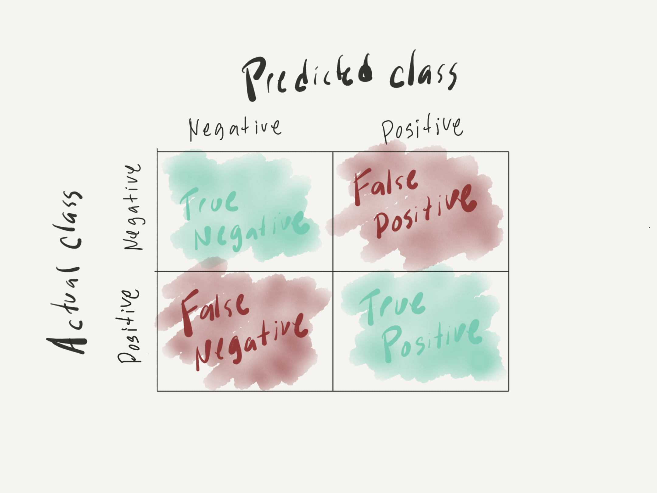
Figure 9.1: Confusion matrix